An official website of the United States government
Here’s how you know
Official websites use .gov A
.gov website belongs to an official government
organization in the United States.
Secure .gov websites use HTTPS A
lock (
) or https:// means you’ve safely connected to
the .gov website. Share sensitive information only on official,
secure websites.
Convection is ongoing across North-Central North Carolina westward into the Appalachians. The upper low is currently centered in eastern Tennessee. The most robust thunderstorms of the afternoon have developed across northwest Carolina along a a boundary extending from NW North Carolina into eastern Kentucky.
Current radar imagery is overlayed with surface dewpoint. Storms are initiating along and north of the boundary.21z forecasted low-level lapse rates from the NAM
The environment is not overly robust to sustain severe convection. Surface-based CAPE values across Northern North Carolina are roughly around 1000 J/Kg with 0-6 km shear 40-50 knots. Low-level lapse rates will be approaching 6-7.5 C/Km by 21z with mid-level lapse rates around 6-7 C/km. The main threat will be marginally severe hail, but 0-3 km helicity values between 150-200 m2/s2 could support a low-end tornado threat. However, as storms move away from the boundary, this threat will decrease.
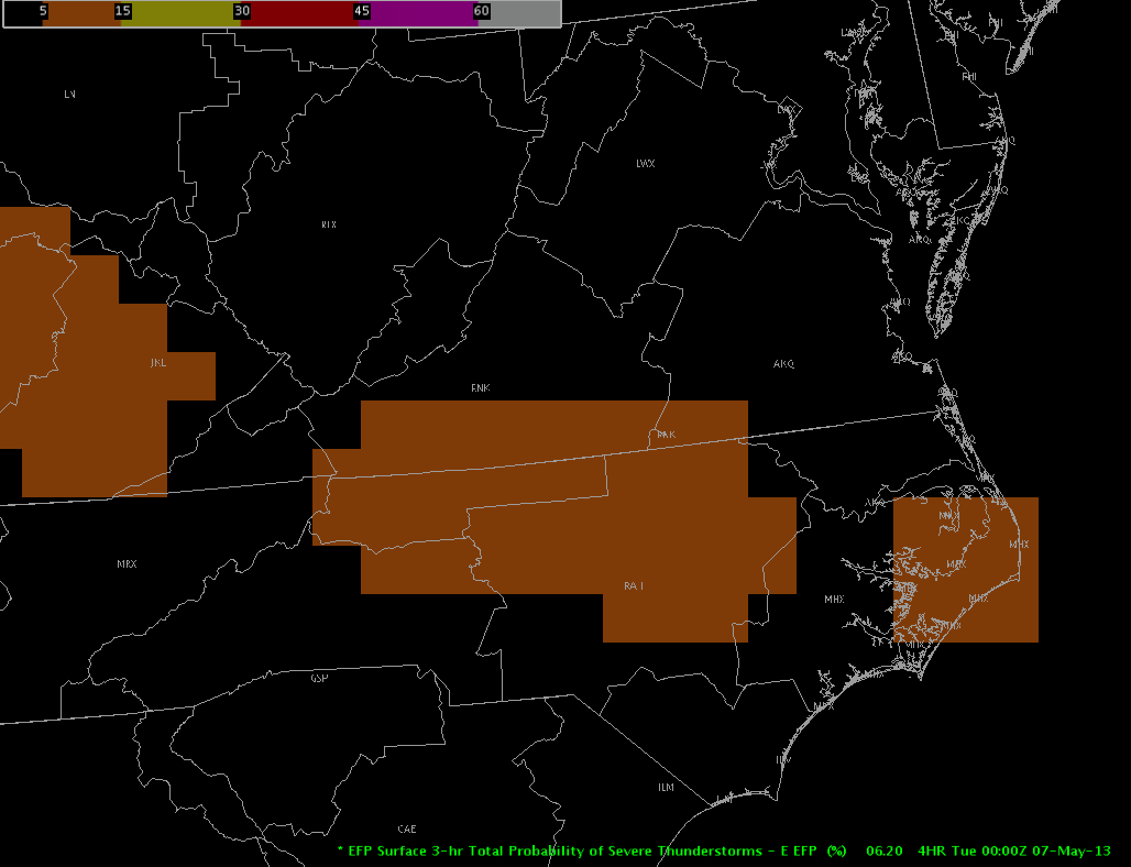
The EFP has placed a 5% probability of severe storms for the previously mentioned area, while a slight risk of severe storms is forecasted by SPC in small area shown in the image below.
Orange color represents a 5% probability of severe weather issued by the EFP.19z Day 1 Outlook from SPC.
As a lobe of energy wraps around the upper-low and moves northward into northern NC, the storms which have already initiated should be able to continue northward into the Blacksburg, VA CWA while some continuing activity is possible across the northwestern extent of the Raleigh, NC CWA.
Monday 6 May 2013 begins the first week of our three-week spring experiment of the 2013 NSSL-NWS Experimental Warning Program (EWP2013) in the NOAA Hazardous Weather Testbed at the National Weather Center in Norman, OK. There will be five primary projects geared toward WFO applications, 1) the development of “best practices” for using Multiple-Radar/Multiple-Sensor (MRMS) severe weather products in warning operations, 2) an evaluation of a dual-polarization Hail Size Discrimination Algorithm (HSDA), 3) an evaluation of model performance and forecast utility of the OUN WRF when operations are expected in the Southern Plains, 4) an evaluation of the Local Analysis Prediction System (LAPS) Space and Time Multiscale Analysis System (STMAS), and 5) an evaluation of multiple CONUS GOES-R convective applications, including pseudo-geostationary lightning mapper products when operations are expected within the Lightning Mapping Array domains (OK, w-TX, AL, DC, FL, se-TX, ne-CO). We will also be coordinating with and evaluating the EFP’s probabilistic severe weather outlooks as guidance for our warning operations. Operational activities will take place during the week Monday through Friday.
For the week of 6-10 May, our distinguished NWS guests will be Marc Austin (WFO Norman, OK), Hayden Frank (WFO Boston, MA), Jonathan Guseman (WFO Lubbock, TX), Nick Hampshire(WFO Fort Worth, TX), Andy Hatzos (WFO Wilmington, OH), and Jonathan Kurtz (WFO Norman, OK). The GOES-R program office, the NOAA Global Systems Divisions (GSD), and NWS WFO Huntsville’s Applications Integration Meteorologist (AIM) Program have generously provided travel stipends for our participants from NWS forecast offices nationwide.
Visiting scientists this week will include Lee Cronce (Univ. Wisconsin), Geoffrey Stano (NASA-SPoRT), Isidora Jankov (NOAA/GSD), and Amanda Terberg (NWS Air Weather Center GOES-R Liaison).
Gabe Garfield will be the weekly coordinator. Clark Payne (WDTB) will be our “Tales from the Testbed” Webinar facilitator. Our support team also includes Darrel Kingfield, Kristin Calhoun, Travis Smith, Chris Karstens, Greg Stumpf, Kiel Ortega, Karen Cooper, Lans Rothfusz, Aaron Anderson, and David Andra.
Each Friday of the experiment (10 May, 17 May, 24 May), from 1200-1240pm CDT, the WDTB will be hosting a weekly Webinar called “Tales From the Testbed”. These will be forecaster-led, and each forecaster will summarize their biggest takeaway from their week of participation in EWP2013. The audience is for anyone with an interest in what we are doing to improve NWS severe weather warnings. New for EWP2013, there will be pre-specified weekly topics. This is meant to keep the material fresh for each subsequent week, and to maintain the audience participation levels throughout the experiment. The weekly schedule:
Week 1: GOES-R; pGLM
Week 2: MRMS, HSDA
Week 3: EFP outlooks, OUN WRF, LAPS
One final post-experiment Webinar will be delivered to the National Weather Association and the Research and Innovation Transition Team (RITT) in June. This Webinar will be a combined effort of both sides of the Hazardous Weather Testbed (EFP and EWP).
Stay tuned on the blog for more information, daily outlooks and summaries, live blogging, and end-of-week summaries as we get underway on Monday 6 May!
1 Apr 2013 marked the first date of the official data collection period for the 2013 experiment.
A few changes this year: 1) data is now available for analysis the next day via the NSSL FTP server (please contact me for access/location), 2) we have added tracking on the flash extent density (many fewer tracked clusters for these cases since we cannot track a storm prior to entering a LMA region), 3) jumps are now calculated not only for the flash rate of a given storm, but also on the max flash extent density (a 1km square within the storm cluster), and also for the flash rate / storm cluster area, and 4) finally, one a major change is the addition of the Earth Networks Total Lightning Network (ENTLN).
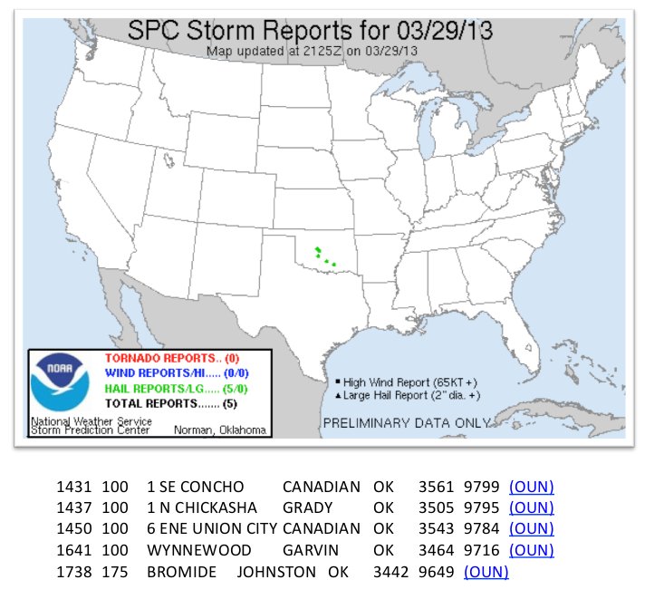
Below is an animated gif from a series of images from the 29 Mar 2013 event over central Oklahoma to illustrate the different products / networks and a few of the issues we’ve seen already (and just prior to start of the “official” data collection).
29 Mar 2013: LMA: initiation locations (diamonds), flash contours (white lines), and flash extent density. KMEANS storm clusters, ID, and past track (Left panel); Earth Networks Total Lightning, KMEANS storm clusters, ID, and past track (top right); NLDN: CG polarity / location and KTLX 0.5 deg Reflectivity (bottom right).
The first thing that should be readily apparent is the differences between detections by the different networks. The LMA provides a location of the flash initiation, the extent of lightning leaders (viewed by Flash Extent Density). The ENTLN provides a lat/lon location of some individual flashes (both in-cloud and cloud-to-ground), though detection efficiency has not been formally established. The NLDN detects primarily cloud-to-ground flashes, providing (lat/lon) locations and polarity.
Here are the jumps (from the various products) from the 29 Mar 2013 event and associated time / cell:
— 1430-1600 UTC jumps (using Ref@-10C to ID and track) —
LMA flash rate: 1438 UTC – cell #288, 1449 UTC – cell #288 LMA max flash density: 1449 UTC – cell #288 LMA flash rate per cluster area (km2): 1438 UTC – cell #288, 1444 UTC – cell #294, 1449 UTC – cell #288 ENTLN flash rate: 1445 UTC – cell #288, 1500 UTC – cell #288
and associated SPC Storm Reports:
First issue in this data set: the central OKLMA was constantly between 5-8 operational stations, contributing to data drop-outs throughout the interesting storm period (note, 6 LMA stations are required to detect any single VHF source point for it to make it past the initial quality control). Obviously, this issue is a concern beyond the OKLMA and today’s data. I am still determining a simple way to flag this issue as part of the xml table output to help the analysis… (more on this below)
Second issue: the server quickly became overloaded and missed creating output files for 3-8 min periods at a time (1540-1830 UTC). We are in the process of determining if we need to load-share with another server or can simply modify some of the data processing. Special note: we have not seen this issue since this event but are constantly watching the load on this server…
———-
The OKLMA definitely has continued to have problems regarding the number of active stations. I’ve included text at the end of this post covering the time period a severe storm (1 in – 2 in hail) crossed over Norman for the case shown below. Included is (ls -al listing of a 10 min period) the file sizes of 10 min of realtime OKLMA raw data files; notice that file size jumps quite wildly from minute to minute. Below that I’ve included the header files from three of those times: 0901, 0903, and 0909 UTC. Each of these minutes have different active stations though only 1 net additional for each time period (11, 12, and 13 active stations, respectfully). But the number of sources detected increases ~exponentially (5, 1919, 5014, respectfully). [Please keep in mind that this is raw VHF source detections and not flashes, the flash sorting occurs later in the processing.]
I believe the addition of the El Reno station at 0903 UTC was key to that increase event detections. I don’t think I’ve seen this drastic of a difference in previous real-time data before. Another reason to, at the very least, add a flag or some type of signifier to the processed data regarding the number of active stations.
(ls -al)
-rw-rw-r– 1 ldm ldm 4456 Mar 31 04:01 LYLOUT_130331_090000_0060.dat
-rw-rw-r– 1 ldm ldm 4384 Mar 31 04:02 LYLOUT_130331_090100_0060.dat
-rw-rw-r– 1 ldm ldm 7274 Mar 31 04:03 LYLOUT_130331_090200_0060.dat
-rw-rw-r– 1 ldm ldm 146025 Mar 31 04:04 LYLOUT_130331_090300_0060.dat
-rw-rw-r– 1 ldm ldm 7574 Mar 31 04:05 LYLOUT_130331_090400_0060.dat
-rw-rw-r– 1 ldm ldm 4382 Mar 31 04:06 LYLOUT_130331_090500_0060.dat
-rw-rw-r– 1 ldm ldm 120348 Mar 31 04:07 LYLOUT_130331_090600_0060.dat
-rw-rw-r– 1 ldm ldm 105323 Mar 31 04:08 LYLOUT_130331_090700_0060.dat
-rw-rw-r– 1 ldm ldm 4977 Mar 31 04:09 LYLOUT_130331_090800_0060.dat
-rw-rw-r– 1 ldm ldm 375058 Mar 31 04:11 LYLOUT_130331_090900_0060.dat
[wdssii@cloudy LMA]$ more LYLOUT_130331_090100_0060.dat
 New Mexico Tech Lightning Mapping Array - analyzed data
 Analysis program: /data1/rtlma/bin/lma_analysis_v10.11.1RT/lma_analysis -d 20130331 -t 090100 -s 60 -l /data1/rtlma/bin/lma_analysis_v10.11.1RT/ok.loc -o /data
 1/rtlma/dec_data/130331/09/01
 Analysis program version: 10.11.1RT
 Analysis started: Sun Mar 31 04:02:20 2013
 Analysis finished: Sun Mar 31 04:02:26 2013
 Data start time: 03/31/13 09:01:00
 Number of seconds analyzed: 60
 Location: OK LMA 2002/2005
 Coordinate center (lat,lon,alt): 35.2791257 -97.9178678 417.90
 Maximum diameter of LMA (km): 194.538
 Maximum light-time across LMA (ns): 649039
 Number of stations: 19
 Number of active stations: 11
 Active stations: C D G H I N Y A U B Z
 Minimum number of stations per solution: 6
 Maximum reduced chi-squared: 5.00
 Maximum number of chi-squared iterations: 20
 Station information: id, name, lat(d), lon(d), alt(m), delay(ns), board_rev, rec_ch
 Sta_info: C Chickasha SE 35.0043455 -97.9073041 339.09 146 3 3
 Sta_info: D Dutton 35.2451748 -98.0754888 420.11 253 3 3
 Sta_info: E El Reno 35.4785046 -98.0089380 419.99 158 3 3
 Sta_info: F FAA 35.3843732 -97.6208285 390.30 52 3 3
 Sta_info: G Goldsby 35.1325178 -97.5185999 382.30 151 3 3
 Sta_info: H Chickasha N 35.1299688 -97.9592651 341.93 159 3 3
 Sta_info: I Minco SE 35.2791257 -97.9178678 417.90 156 3 3
 Sta_info: M Middleberg 35.1347342 -97.7257633 414.68 159 3 3
 Sta_info: N Newcastle 35.2564446 -97.6589268 396.65 155 3 3
 Sta_info: O OKC 35.4015724 -97.6014842 393.99 119 3 3
 Sta_info: W Minco W 35.3622021 -98.0397279 415.65 158 3 3
 Sta_info: Y Yukon 35.4402883 -97.7782383 405.96 162 3 3
 Sta_info: A Altus Airport 34.6966400 -99.3406100 435.60 148 3 3
 Sta_info: P Prairie Hill 34.5950200 -99.4936800 447.40 159 3 3
 Sta_info: U Mangum 34.8592300 -99.3612100 483.10 174 3 3
 Sta_info: B Bluff 34.7679400 -99.5392400 509.60 234 3 3
 Sta_info: O Olustee 34.5195200 -99.4349400 407.50 157 3 3
 Sta_info: R Granite 34.9733400 -99.4487200 492.90 168 3 3
 Sta_info: Z Zombie 34.7116100 -99.0802600 427.90 159 3 3
 Station data: id, name, win(us), dec_win(us), data_ver, rms_error(ns), sources, %, <P/P_m>, active
 Sta_data: C Chickasha SE 80 10 70 2 40.0 1.77 A
 Sta_data: D Dutton 80 10 70 3 60.0 9.30 A
 Sta_data: E El Reno 0 0 70 0 0.0 0.00 NA
 Sta_data: F FAA 0 0 70 0 0.0 0.00 NA
 Sta_data: G Goldsby 80 10 70 5 100.0 0.88 A
 Sta_data: H Chickasha N 80 10 70 4 80.0 3.71 A
 Sta_data: I Minco SE 80 10 70 0 0.0 0.00 A
 Sta_data: M Middleberg 0 0 70 0 0.0 0.00 NA
 Sta_data: N Newcastle 80 10 70 4 80.0 0.99 A
 Sta_data: O OKC 0 0 70 0 0.0 0.00 NA
 Sta_data: W Minco W 0 0 70 0 0.0 0.00 NA
 Sta_data: Y Yukon 80 10 70 3 60.0 2.48 A
 Sta_data: A Altus Airport 80 10 70 1 20.0 0.06 A
 Sta_data: P Prairie Hill 0 0 70 0 0.0 0.00 NA
 Sta_data: U Mangum 80 10 70 2 40.0 0.35 A
 Sta_data: B Bluff 80 10 70 3 60.0 1.06 A
 Sta_data: O Olustee 0 0 70 0 0.0 0.00 NA
 Sta_data: R Granite 0 0 70 0 0.0 0.00 NA
 Sta_data: Z Zombie 80 10 70 3 60.0 0.08 A
 Metric file version: 4
 Station mask order: ZROBUPAYWONMIHGFEDC
 Data: time (UT sec of day), lat, lon, alt(m), reduced chi^2, P(dBW), mask
 Data format: 15.9f 12.8f 13.8f 9.2f 6.2f 5.1f 7x
 Number of events: 5
 *** data ***
 32483.420073930 33.10235512 -100.69250915 450975.32 2.11 36.6 0x01932
 32492.744501099 34.85556274 -98.92710217 43824.93 1.60 20.7 0x4c032
 32497.223350796 35.13756612 -97.95587964 1403.88 0.83 18.8 0x04133
 32504.743797217 35.44091271 -97.67734666 45462.14 4.07 23.5 0x48911
 32506.247514080 31.47113948 -99.42825852 425506.86 4.15 36.4 0x48930
———————–
[wdssii@cloudy LMA]$ more LYLOUT_130331_090300_0060.dat
 New Mexico Tech Lightning Mapping Array - analyzed data
 Analysis program: /data1/rtlma/bin/lma_analysis_v10.11.1RT/lma_analysis -d 20130331 -t 090300 -s 60 -l /data1/rtlma/bin/lma_analysis_v10.11.1RT/ok.loc -o /data
 1/rtlma/dec_data/130331/09/03
 Analysis program version: 10.11.1RT
 Analysis started: Sun Mar 31 04:04:20 2013
 Analysis finished: Sun Mar 31 04:04:39 2013
 Data start time: 03/31/13 09:03:00
 Number of seconds analyzed: 60
 Location: OK LMA 2002/2005
 Coordinate center (lat,lon,alt): 35.2791257 -97.9178678 417.90
 Maximum diameter of LMA (km): 194.538
 Maximum light-time across LMA (ns): 649039
 Number of stations: 19
 Number of active stations: 12
 Active stations: C D E G H I N Y P U R Z
 Minimum number of stations per solution: 6
 Maximum reduced chi-squared: 5.00
 Maximum number of chi-squared iterations: 20
 Station information: id, name, lat(d), lon(d), alt(m), delay(ns), board_rev, rec_ch
 Sta_info: C Chickasha SE 35.0043455 -97.9073041 339.09 146 3 3
 Sta_info: D Dutton 35.2451748 -98.0754888 420.11 253 3 3
 Sta_info: E El Reno 35.4785046 -98.0089380 419.99 158 3 3
 Sta_info: F FAA 35.3843732 -97.6208285 390.30 52 3 3
 Sta_info: G Goldsby 35.1325178 -97.5185999 382.30 151 3 3
 Sta_info: H Chickasha N 35.1299688 -97.9592651 341.93 159 3 3
 Sta_info: I Minco SE 35.2791257 -97.9178678 417.90 156 3 3
 Sta_info: M Middleberg 35.1347342 -97.7257633 414.68 159 3 3
 Sta_info: N Newcastle 35.2564446 -97.6589268 396.65 155 3 3
 Sta_info: O OKC 35.4015724 -97.6014842 393.99 119 3 3
 Sta_info: W Minco W 35.3622021 -98.0397279 415.65 158 3 3
 Sta_info: Y Yukon 35.4402883 -97.7782383 405.96 162 3 3
 Sta_info: A Altus Airport 34.6966400 -99.3406100 435.60 148 3 3
 Sta_info: P Prairie Hill 34.5950200 -99.4936800 447.40 159 3 3
 Sta_info: U Mangum 34.8592300 -99.3612100 483.10 174 3 3
 Sta_info: B Bluff 34.7679400 -99.5392400 509.60 234 3 3
 Sta_info: O Olustee 34.5195200 -99.4349400 407.50 157 3 3
 Sta_info: R Granite 34.9733400 -99.4487200 492.90 168 3 3
 Sta_info: Z Zombie 34.7116100 -99.0802600 427.90 159 3 3
 Station data: id, name, win(us), dec_win(us), data_ver, rms_error(ns), sources, %, <P/P_m>, active
 Sta_data: C Chickasha SE 80 10 70 1841 95.9 3.53 A
 Sta_data: D Dutton 80 10 70 67 3.5 1.62 A
 Sta_data: E El Reno 80 10 70 1876 97.8 1.11 A
 Sta_data: F FAA 0 0 70 0 0.0 0.00 NA
 Sta_data: G Goldsby 80 10 70 1888 98.4 1.41 A
 Sta_data: H Chickasha N 80 10 70 78 4.1 0.65 A
 Sta_data: I Minco SE 80 10 70 17 0.9 0.00 A
 Sta_data: M Middleberg 0 0 70 0 0.0 0.00 NA
 Sta_data: N Newcastle 80 10 70 1868 97.3 1.18 A
 Sta_data: O OKC 0 0 70 0 0.0 0.00 NA
 Sta_data: W Minco W 0 0 70 0 0.0 0.00 NA
 Sta_data: Y Yukon 80 10 70 30 1.6 5.42 A
 Sta_data: A Altus Airport 0 0 70 0 0.0 0.00 NA
 Sta_data: P Prairie Hill 80 10 70 1909 99.5 0.00 A
 Sta_data: U Mangum 80 10 70 17 0.9 0.18 A
 Sta_data: B Bluff 0 0 70 0 0.0 0.00 NA
 Sta_data: O Olustee 0 0 70 0 0.0 0.00 NA
 Sta_data: R Granite 80 10 70 20 1.0 0.49 A
 Sta_data: Z Zombie 80 10 70 1908 99.4 0.42 A
 Metric file version: 4
 Station mask order: ZROBUPAYWONMIHGFEDC
 Data: time (UT sec of day), lat, lon, alt(m), reduced chi^2, P(dBW), mask
 Data format: 15.9f 12.8f 13.8f 9.2f 6.2f 5.1f 7x
 Number of events: 1919
 *** data ***
 32580.015923202 35.30497068 -98.02190064 7436.24 1.23 16.2 0x42115
 32580.028474879 35.03748360 -97.48952779 7700.38 0.15 16.4 0x42115
————————————–
[wdssii@cloudy LMA]$ more LYLOUT_130331_090900_0060.dat
 New Mexico Tech Lightning Mapping Array - analyzed data
 Analysis program: /data1/rtlma/bin/lma_analysis_v10.11.1RT/lma_analysis -d 20130331 -t 090900 -s 60 -l /data1/rtlma/bin/lma_analysis_v10.11.1RT/ok.loc -o /data1/rtlma
 /dec_data/130331/09/09
 Analysis program version: 10.11.1RT
 Analysis started: Sun Mar 31 04:10:20 2013
 Analysis finished: Sun Mar 31 04:10:56 2013
 Data start time: 03/31/13 09:09:00
 Number of seconds analyzed: 60
 Location: OK LMA 2002/2005
 Coordinate center (lat,lon,alt): 35.2791257 -97.9178678 417.90
 Maximum diameter of LMA (km): 194.538
 Maximum light-time across LMA (ns): 649039
 Number of stations: 19
 Number of active stations: 13
 Active stations: C D E G H I N W Y P U R Z
 Minimum number of stations per solution: 6
 Maximum reduced chi-squared: 5.00
 Maximum number of chi-squared iterations: 20
 Station information: id, name, lat(d), lon(d), alt(m), delay(ns), board_rev, rec_ch
 Sta_info: C Chickasha SE 35.0043455 -97.9073041 339.09 146 3 3
 Sta_info: D Dutton 35.2451748 -98.0754888 420.11 253 3 3
 Sta_info: E El Reno 35.4785046 -98.0089380 419.99 158 3 3
 Sta_info: F FAA 35.3843732 -97.6208285 390.30 52 3 3
 Sta_info: G Goldsby 35.1325178 -97.5185999 382.30 151 3 3
 Sta_info: H Chickasha N 35.1299688 -97.9592651 341.93 159 3 3
 Sta_info: I Minco SE 35.2791257 -97.9178678 417.90 156 3 3
 Sta_info: M Middleberg 35.1347342 -97.7257633 414.68 159 3 3
 Sta_info: N Newcastle 35.2564446 -97.6589268 396.65 155 3 3
 Sta_info: O OKC 35.4015724 -97.6014842 393.99 119 3 3
 Sta_info: W Minco W 35.3622021 -98.0397279 415.65 158 3 3
 Sta_info: Y Yukon 35.4402883 -97.7782383 405.96 162 3 3
 Sta_info: A Altus Airport 34.6966400 -99.3406100 435.60 148 3 3
 Sta_info: P Prairie Hill 34.5950200 -99.4936800 447.40 159 3 3
 Sta_info: U Mangum 34.8592300 -99.3612100 483.10 174 3 3
 Sta_info: B Bluff 34.7679400 -99.5392400 509.60 234 3 3
 Sta_info: O Olustee 34.5195200 -99.4349400 407.50 157 3 3
 Sta_info: R Granite 34.9733400 -99.4487200 492.90 168 3 3
 Sta_info: Z Zombie 34.7116100 -99.0802600 427.90 159 3 3
 Station data: id, name, win(us), dec_win(us), data_ver, rms_error(ns), sources, %, <P/P_m>, active
 Sta_data: C Chickasha SE 80 10 70 4319 86.1 2.37 A
 Sta_data: D Dutton 80 10 70 84 1.7 7.58 A
 Sta_data: E El Reno 80 10 70 4455 88.9 0.91 A
 Sta_data: F FAA 0 0 70 0 0.0 0.00 NA
 Sta_data: G Goldsby 80 10 70 4070 81.2 1.26 A
 Sta_data: H Chickasha N 80 10 70 149 3.0 1.27 A
 Sta_data: I Minco SE 80 10 70 38 0.8 0.00 A
 Sta_data: M Middleberg 0 0 70 0 0.0 0.00 NA
 Sta_data: N Newcastle 80 10 70 4562 91.0 1.05 A
 Sta_data: O OKC 0 0 70 0 0.0 0.00 NA
 Sta_data: W Minco W 80 10 70 4128 82.3 5.69 A
 Sta_data: Y Yukon 80 10 70 95 1.9 3.14 A
 Sta_data: A Altus Airport 0 0 70 0 0.0 0.00 NA
 Sta_data: P Prairie Hill 80 10 70 4804 95.8 0.00 A
 Sta_data: U Mangum 80 10 70 47 0.9 0.08 A
 Sta_data: B Bluff 0 0 70 0 0.0 0.00 NA
 Sta_data: O Olustee 0 0 70 0 0.0 0.00 NA
 Sta_data: R Granite 80 10 70 60 1.2 0.22 A
 Sta_data: Z Zombie 80 10 70 4368 87.1 0.32 A
 Metric file version: 4
 Station mask order: ZROBUPAYWONMIHGFEDC
 Data: time (UT sec of day), lat, lon, alt(m), reduced chi^2, P(dBW), mask
 Data format: 15.9f 12.8f 13.8f 9.2f 6.2f 5.1f 7x
 Number of events: 5014
 *** data ***
 32940.000377496 35.03210068 -97.80952546 4892.64 0.47 17.7 0x42515
 32940.014071929 35.06811963 -97.21688673 4949.58 1.00 16.3 0x02515
Since a blog presents stories in reverse chronological order, those new coming into the blog will find my most recent stories first, even though they are intended to be later chapters. So, here is a chronological table of contents of the Experimental Warning Thoughts. I’ll update this and bump it to the top every once in a while.
As finally promised as an “aside” in this blog entry, I will cover the issue of how using point observations can lead to a misrepresentation of the lead time of a warning.
Consider that one warning is issued, and a single severe weather report is received for that warning. We have a POD = 1 (one report is warning, zero are unwarned), and an FAR = 0 (one warning is verified, zero warnings are false). Nice!
How do we compute the lead time for this warning? Presently, this is done by simply subtracting the warning issuance time from the time of the first report on the storm. From this earlier blog post:
twarningBegins = time that the warning begins
twarningEnds= time that the warning ends
tobsBegins = time that the observation begins
tobsEnds= time that the observation ends
LEAD TIME (lt): tobsBegins – twarningBegins [HIT events only]
For ease of illustration, I’m using the spatial scale to represent the time scale. The warning begins at some time twarningBegins, and the report is at a later time tobsBegins. The lead time is shown spatially in the figure, and in this case, it appears that the warning was issued with some appreciable lead time before the event at the reporting location occurs.
However, as we explained in the previous blog post, reports only represent a single sample of the severe weather event in space in time. How can we be certain that the report above represents the location and time of the very first instance that the storm became severe? In all but probably rare cases, it does not, and the storm became severe at some time prior to the time of that report. This tells us that for pretty much every warning (hail and wind events at least), the computed lead times are erroneously too large! Reality looks more like this:
ADDENDUM (1/10/2013): Here is another way to view this so that the timeline of events is better illustrated. In this next example, a warning is issued at t=0 minutes on a storm that is not yet severe, but expected to become severe in the next 10-20 minutes, hence hopefully providing that amount of lead time. Let’s assume that the red contour in the storm indicates the area over which hail >1″ is falling, and when red appears, the storm is officially severe. As the storm moves east, I’ve “accumulated” the severe hail locations into a hail swath (much like the NSSL Hail Swath algorithm works using multiple-radar/multiple-sensor data). Only two storm reports were received on this storm, one at t=25 minutes after the warning was issued, and another at t=35 minutes. That means this warning verified (was not a false alarm), and both reports were warned (two hits, no misses). The lead times for each report were 25 and 35 minutes respectively, but official warning verification uses lead time to the first report known as the initial lead time. Therefore, the lead time recorded for this warning would be 25 minutes, which is very respectable. However, in this case, the storm was actually severe starting at t=10 minutes. The lead time between the start of the warning and the start of severe weather was 15 minutes shorter than that officially recorded.
How can we be more certain of the actual lead times of our warnings? By either gathering more reports on the storm (which isn’t always entirely feasible, although that may be improving with new weather crowdsourcing apps like mPING), or using proxy verification based on a combination of remotely-sensed data (like radar data) and actual reports. Again, more on this later…
I’m back after a too-lengthy absence from this blog. I’ve been thinking about some experimental warning issues again lately, and have a few things to add to the blog regarding some more pitfalls of our current warning verification methodology. I hinted on these in past posts, but would like to expand upon them.
Have you ever been amazed that some especially noteworthy severe weather days can produce record numbers of storm reports? Let’s take this day for example, 1 July 2012:
Wow! A whopping 522 wind reports and 212 hail reports. That must have been an exceptionally-bad severe weather day. (It actually was the day of the big Ohio Valley to East Coast derecho from last July, a very impactful event).
But what makes a storm report? Somebody calls in, or uses some kind of software (e.g., Spotter Network), to report that the winds were X mph or the hail was Y inches in diameter from some location and at some time from within the severe thunderstorm. But the severe weather event is actually impacting an area surrounding the location from which the report was generated, and has been and will occur over the time interval representing the lifetime of the storm. It is highly unlikely that a hail report represented only a single stone falling at that location, or that the wind report represented a single wind gust local to that single location, and there were no other severe wind gusts anywhere else nor at any other time during the storm. Each of these reports represent only a single sample of an event that covers a two-dimensional space over a time period.
If you recall from this blog entry, the official Probability Of Detection (POD) is computed to be the number of reports that were within warning polygons over the total number of reports (inside and outside polygons). It’s easy to see that to effectively improve a office’s overall POD for a time period (e.g., one year), they only need to increase the number of reports that are covered by the warning polygons issued by that office during that time period. One way to do this is to cast a wide net, and issue larger and longer-duration warning polygons. But another way to artificially improve POD is to simply increase the number of reports within storms via aggressive report gathering. Let’s consider a severe weather event like this one:
Look at all those (presumably) severe-sized hail stones. We can make a report on each one, at each time they fell. After about an hour of counting and collecting (before they all melted), this observer found 5,462 hail stones that were greater than 1″ in diameter. Beautiful – the Probability Of Detection is going to go way up! We can also count all the damaged trees as well to add hundreds of wind reports. Do you see the problem here? Are you getting tired of my extrapolations to infinity? Yes, there are literally an infinite number of severe weather reports that can be gleaned from this event (technically, there is a finite number of severe-size hail stones fell in this storm, but who’s really counting that gigantic number?). But let’s scale this back. Here’s a scenario in which a particular warning is verified two different ways:
Each warning polygon verifies, so no false alarms. For the scenario on the top, there is one hit added to all reports for the time period (maybe a year’s worth of warning), but for the bottom scenario, there are seven hits added to the statistics.
But wait, doesn’t the NWS Verification Branch filter storm reports that are in close proximity in space and time when computing warning statistics? Wouldn’t those seven hits be reduced to a smaller amount? They use a filter of 10 miles and 15 minutes to avoid my hypothetical over-reporting scenario. But that really doesn’t address the issue entirely. One can still try to fill every 10 mile and 15 minute window with a hail or wind report in order to maximize their POD. But if you think about it, that’s not really a bad idea. In essence, you are filling a grid with a 10 mile and 15 minute resolution with as much information known about the storm as possible. But this works only if you also call into every 10-miles/15-minute grid point inside and outside every storm. Forecasters rarely do this (and realistically can’t), because of workload issues, and because only one report within a warning polygon is all that is needed to avoid that warning from being labelled a false alarm (again, cast the wide net so that one can increase their chance of getting a report within the warning).
CORRECTION (1/10/2013): I just learned that the 10 mile / 15 minute filtering was only done in the era of county-based warning verification, and is not done for storm-based verification. Therefore, my arguments against the current verification methodology where hit rates and POD can be stacked by gathering more storm reports is further bolstered. More information is in the NWS Directive on forecast and warning verification.
If we knew exactly what was happening within the storm at all times and locations at every grid point (in our case, every 1 km and 1 minute), we’d have a very robust verification grid to use for the geospatial warning verification methodology. But we really don’t know exactly what’s is happening everywhere all the time because it is nearly impossible to collect all those data points. The Severe Hazards Analysis and Verification Experiment (SHAVE) is attempting to improve on the report density in time and space. But their resources are also finite, and they don’t have the staffing to call into every thunderstorm. Their high-resolution data set is very useful, but limited to only the storms they’ve called. What could we do to broaden the report database so that we have a better idea of the full scope of the impact of every storm? One concept is proxy verification, in which some other remotely-sensed method is used to make a reasonable approximation of the coverage of severe weather within a storm, like so:
This set of verification data will have a degree of uncertainty associated with it, but the probability of the event isn’t zero, and is thus, useful. It is also very amenable to the geospatial verification methodology already introduced in this blog series. More on this later…
Finally, a bit more activity in some of our domains this week. In the last couple hours widespread severe (and near severe) storms have developed across the WTLMA. Activity is expected to continue in the SW OKLMA network and possibly central OK later tonight. SHAVE is currently actively calling in the region west and NW of Lubbock, reporting primarily pea-to-dime-size hail (severe winds are likely to be a larger factor with these storms) .
Above image is screen capture of realtime webpage active using google maps at 2231 UTC on 26 Sept 2012. Storms with jumps are noted, image shows timing & flash rate at that time (total per min & CG per 5 min) for storms tracked using Scale 1 (data for storm tracking at smaller and larger scales also available). SHAVE data collection points are denoted by green (0.25-0.75 in hail) and grey (no hail) circles.
Data collection update:
17 Sept 2012: NALMA 2000-2200 UTC (severe possibly out-of-range)
18 Sept 2012: DCLMA 1430-2230 UTC
25 Sept 2012: OKLMA 2300-0400 UTC (SHAVE data available)
26 Sept 2012: WTLMA/ OKLMA 1900 – ? (SHAVE data available)
Relatively quiet weather has continued over the domains during the last week. Today’s event over the NALMA is likely to be primarily a heavy rain event, but it’s still a good opportunity to show how the same storm system is tracked simultaneously at different scales. For the LJA, we are running 3 scales concurrently: scale 0 (200 km^2 min cluster size), scale 1 (600 km^2), and scale 2 (1000 km^2):
Scale 0 over the NALMA domain. Clusters are the regions identified by the colorful shapes over the reflectivity at -10 C plot.similar to the previous image, except for Scale 1. similar to the previous images, except for Scale 2. At scale 2, the identified storm clusters are allowed to grow unbounded.
(severe, or near severe) events since last update:
This week has been a bit more active than we’ve seen in recent weeks… In fact, currently the storm in SW Oklahoma county just produced two lightning jumps (2021/2024 & 2030 UTC) about the same time that radar velocity indicated the start of a downburst…
Lightning jump associated with storm over SW Oklahoma county at 2024 UTC. Top row of table includes values for this cell (#403352). Right panel shows tracked region selected at smallest scale (scale 0). Note: scale 1 & 2 were not tracking storms over the region due to size requirements. i.e., these storms were too small.TDWR velocity at 2027 UTC over southwest Oklahoma county.
Activity has also occurred in other regions as well this week. Below is a breakdown of (severe/near severe activity):
2 Sept 2012: NALMA 1900-0300 UTC
5 Sept 2012: WTLMA/OKLMA (sw) 2330-0300 UTC
6 Sept 2012: DCLMA 1030-1330 UTC
7 Sept 2012: OKLMA 2000-? UTC
We’re still actively collecting data. Activity has been rather minimal across the networks for the last couple weeks (SHAVE has been down since the start of the new semester).
Hurricane Isaac made landfall last week, primarily affecting regions outside the LMA domains. Convective rain bands moved over the FL-LDAR network on 27 Aug, though they produced very little lightning (the MLB office had 2 preliminary storm reports for the day though likely in regions out-of-range of the FL-LDAR system).
Severe storms occurred over the northern Alabama network on 2 Sept 2012 as the remnants of Isaac moved eastward out of Arkansas and into the Tennessee Valley. 21 preliminary severe wind reports were recorded in the Huntsville county warning area with these storms.
Summary since last blog post:
24-25 Aug 2012: WTLMA, 0300-0600 UTC (25th)
25 Aug 2012: OKLMA/WTLMA, 2100-0200 UTC
26 Aug 2012: DCLMA, 1700-1900 UTC
27 Aug 2012: FL-LDAR (likely out-of-range), 1400-1600 UTC