
Geospatial warning verification addresses both of the pitfalls explained in earlier blog entries by consolidating the verification measures into one 2×2 contingency table. The verified hazards can be treated as two-dimensional areas, of which they are – storm hazards do not affect just points or lines! We can include the correct null forecasts in the measures. This method provides a more robust way to determine location-specific lead times as well as new metrics known as departure time and false time. In addition, the method will reward spatial and temporal precision in warnings and penalize “casting a wider net” by measuring false alarm areas and false alarm times, which may contribute to a high false alarm perception by the public.
How might we measure the effect of the last issue addressed? Let’s take our Tuscaloosa example and see what the effect of varying the warning size and duration has on our verification numbers. I will only present a few test cases here, because I want to eventually explore this further with a different storm case that isn’t comprised of a single long-tracked isolated storm.
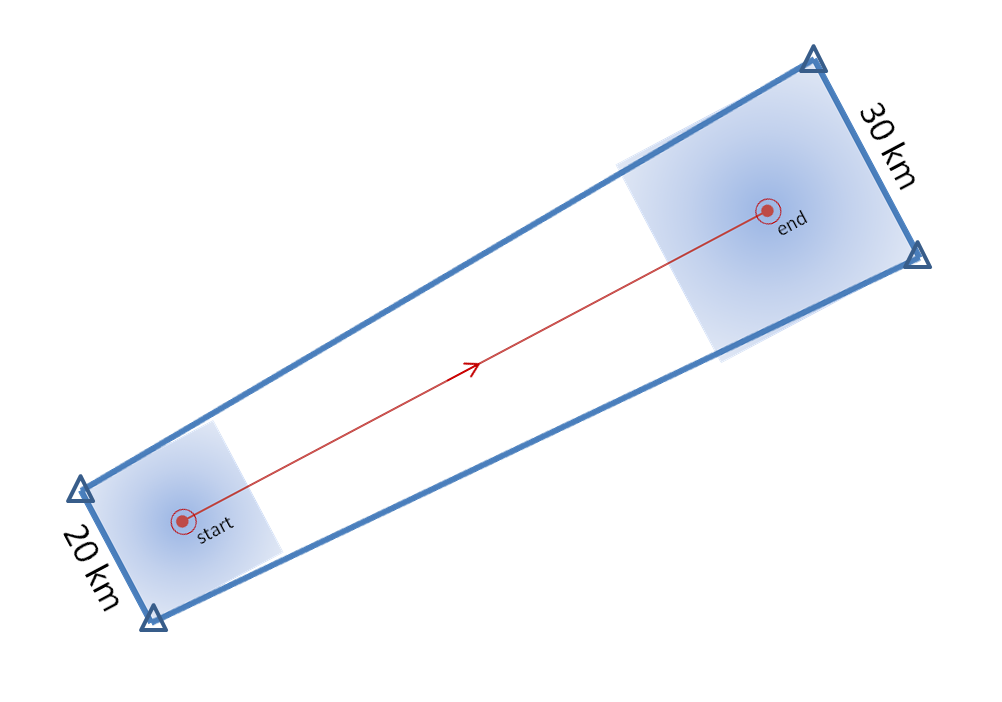
I developed a method which will take my truthed mesocyclone centroid locations and use them to compute the storm motion vector as specific warning decision points along the storm track. Starting from the initial warning decision point from the BMX WFO on the TCL storm (2038 UTC 27 April 2011), I created warning polygons using the default AWIPS WarnGen polygon shape parameters. Namely, the current threat point is projected to its final position using the motion vector and a prescribed warning duration. A 10 km buffer is drawn around the starting threat point resulting in the back edge of the warning being 20km. A 15 km buffer is drawn around the ending threat point resulting in the back edge of the warning being 30km. The far corners of each box are then connected to create the trapezoid shape of the default warning polygon.
I used a 60-minute warning duration since the NWS warnings were also about 60 minutes in duration for the TCL storm. I have a re-warning interval of 60 minutes, so that a new warning polygon is issued as the hazard location is nearing the downstream end of the current warning polygon. Because of the buffer around the projected ending point of the threat, each successive warning will have some overlap with the previous warning, which is considered a best warning practice. None of the warnings will be edited for shape based on any county border, because we want to test the effect of warning size and duration without any other factors influencing the warning area. A loop of the warning polygons with the mesocyclone path overlaid:
Here is the 2×2 table using a 5 km radius of influence (“splat”) around the one-minute tornado observations, I am not applying the Cressman distance weighting to the truth splats, and I’m using the composite reflectivity filtering for the correct nulls:
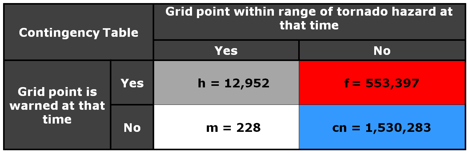
And the grid point method scores are:
POD = 0.9827
FAR = 0.9771
CSI = 0.0229
The FAR and CSI are slightly better than the NWS warnings. However, I’m not trying to compare this method to the actual warnings, but rather as a start to determine the effect of larger and longer warning polygons. So, let’s try that now. Instead of using starting and ending box sizes of 20 and 30 km respectively for our default WarnGen polygon, let’s cast a wider net and quadruple that to 80 and 120 km. The polygon loop would look like this:
And the 2×2 table and scores like this:

POD =1.0000
FAR = 0.9962
CSI =0.0038
What was the effect of the larger longer polygons? Well first, there were no missed grid points, and the POD = 1. But the number of false alarm grid points increased by a factor of about 7, and thus the FAR went up and the CSI went down. Recall that the number of false alarm grid points represents the number of 1 km2 grid points accumulated for each minute of data, so the false alarm area and time are much larger, even though these warnings verified perfectly.
So let’s take this in the opposite direction and make our warning polygons smaller. We’ll use starting and ending box sizes of 6 and 10 km respectively. The loop:
and the numbers:

POD = 0.6668
FAR = 0.9422
CSI =0.0561
We’ve significantly reduced the false alarm area, but we also negatively affected the POD. About 1/3 of the tornado grid points were missed because the warnings were too small.
Now, let’s run the “Truth Event” statistics on all three scenarios:
3 km: pod 0.6390, far 0.3041, csi 0.4995, hss 0.6563, lt 32.8, dt 27.4, ft 61.8
10 km: pod 0.9968, far 0.6780, csi 0.3217, hss 0.4619, lt 39.0, dt 32.1, ft 71.3
40 km: pod 1.0000, far 0.9164, csi 0.0836, hss 0.1015, lt 73.2, dt 46.7, ft 114.6
The 3 km warnings have the best CSI and HSS. This appears that the geospatial verification scheme is rewarding more precise polygons. But there is a problem…there is also a pretty low POD, which means that portions of the tornadoes are not being warned. That’s not good, and reflective of the Doswell “asymmetric penalty function” where forecasters are harmed more by missed tornadoes than false alarms. Why is this so? Because our warnings are being issued for 60 minute durations and 60-minute re-warning intervals. That means for these narrow warnings, if the storm motion deviates after the warning is issued, then there is no chance to re-adjust the warning to account for the storm motion changes. Hence, a larger warning would capture these changes.
One might wonder – how can we balance precision and high POD? I will treat this issue in a later blog, but for now, the next entry will continue to look at the issues of casting a wider net as it pertains to a very hot topic right now – how to warn for Quasi-Linear Convective System (QLCS) tornadoes.
Greg Stumpf, CIMMS and NWS/MDL
