We will now introduce a new approach to creating convective weather hazard information which was first tested at the NOAA Hazardous Weather Testbed (HWT) with visiting NWS forecasters in 2007 and 2008.  The new warning methodology varies in complexity and flexibility, but we will first present the basic concepts first.  In this approach, the forecaster still determines a motion vector and chooses a warning duration.  However, instead of tracking points and lines, the forecaster outlines the probable severe weather threat area at the current time, and inputs motion uncertainty.  From this information are derived high-resolution rapidly-updating geospatial digital hazard grids.  These grids are used to generate a wide variety of useful warning information, including warning swaths over a time period, meaningful information for time of arrival and departure for any location within the warned area, and probabilistic information based on the storm motion uncertainty.

First, let’s tackle the subject of this entry, “let’s get digital”.  Right now, the official warning products are still transmitted as an ASCII text product, and all the pertinent numerical information in the warning like begin and end times, polygon lat/lon coordinates, and other information needs to be “parsed” out of the text product in order for various applications to take advantage of them (e.g., iNWS mobile alerting).  This is an archaic method to deliver information, especially in this day and age of digital technology.  Various options are being explored to improve the data delivery method, including encoding the warning information into the Common Alerting Protocol (CAP) format.  While we feel this is an improvement, it is not going to be sufficient to completely convey all the possible modes of hazard information that can be created and delivered.  For example, the polygon information is still encoded as a series of lat/lon points within the CAP formatted files.  But what if the polygon is comprised of complex boundaries or curved edges?  Or what if we want to include intermediate threat area information at specific times steps during the warning?  Considering that we’ve made the argument for gridded warning verification, we feel that hazard information should be presented as a digital grid, more easily exploitable by today’s technology.  You’ll understand why in a little bit…

So first addressing how a forecaster determines a current threat, instead of choosing points or lines and trying to decide where to place these points within the storm hazard areas, we feel that the warnings should be based on the tracking of a threat area.  Here are the proposed steps in this new warning process.  For each step, I’ve also added a snippet of ideas for “more sophistication” that I may explore further in later blog entries.

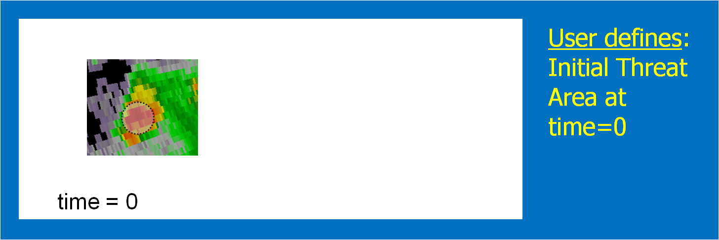
1.  The forecaster outlines the current threat area.

For our HWT exercises, we gave the forecaster two options, a) draw a free-hand multi-sided polygon, or b) fit the current threat area with and ellipse.  (The latter was offered because it is easier to project an area described by a known mathematical function, than it is for a free-hand polygon area).  Where is the threat outline drawn?  That is currently up to the forecaster to make their best determination where the severe weather currently resides in the storm.  They can make use of radar and other data as well as algorithms for their decisions.  Fig. 1 illustrates an initial threat area defined as a circular area.  A circle is chosen to illustrate the effect of some of the later concepts below.

[More sophistication:  The threat area is currently a deterministic contour (inside = yes or 100%, outside = no or 0%), but because we are entering data digitally, this initial threat area could be a probabilistic grid.  For now, to keep it simple, we’ll just go with “you’re either in or you’re out”.]

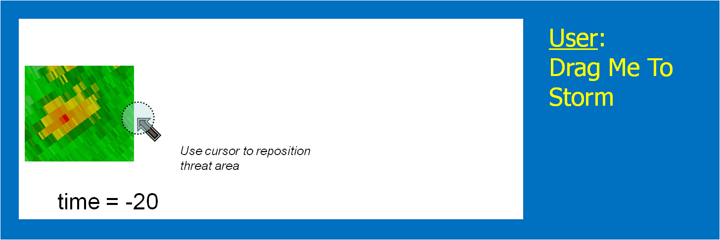
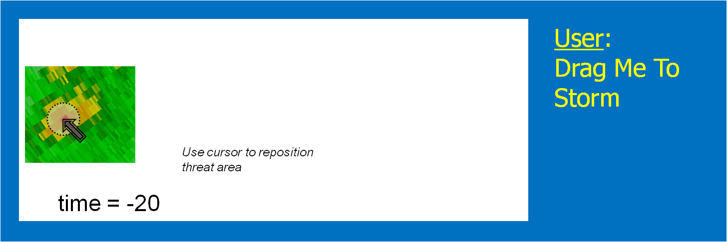
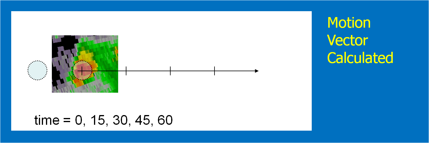
2.  Determine the threat motion vector.

The motion vector could be determined using today’s WarnGen method of “Drag Me To Storm”.  This is done by finding a representative location in the storm to track on the current radar volume scan, and then stepping back to a past volume scan (Fig. 2; 20 minutes in the past) and dragging the point to the same feature (Fig. 3).  The distance and orientation between the current and past points would define the motion vector (Fig. 4).  This is how we did it during our HWT exercises.

[More sophistication:  Determine the motion vector by stepping the radar data back in time and repeating the process in step 1, drawing another threat hazard area.  Then, an application such as the K-Means segmentation algorithm developed by NSSL could determine the motion vector betwen the two threat areas, or even a high-resolution two-dimensional motion field.]

3.  Choose a warning duration.

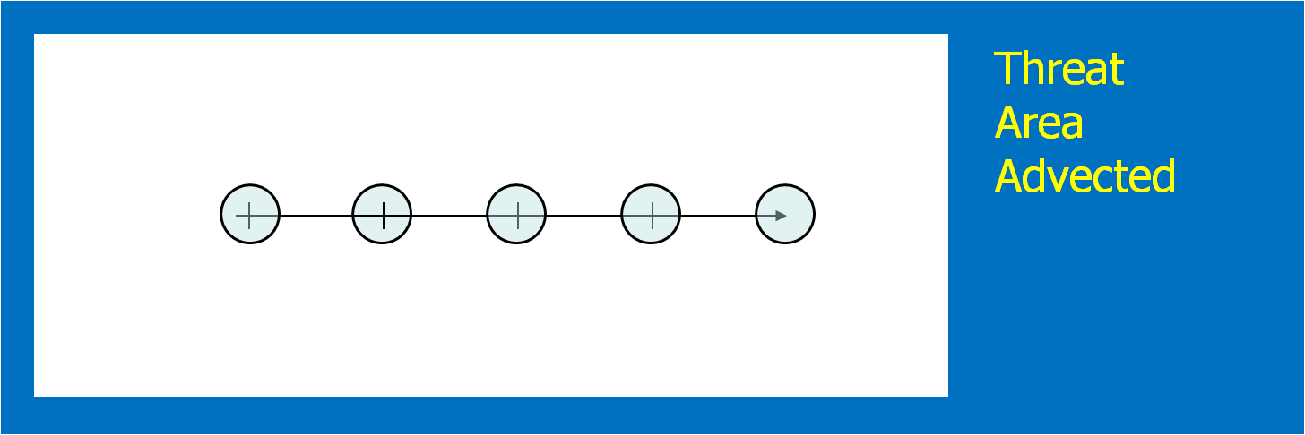
This is usually easy – how long does the forecaster want the warning to extend.   The initial threat area is then projected to the final position.  In addition, the threat area is projected to every time step between the warning issuance time and the warning duration time.  We used a time interval of one minute in the HWT experiment.  Figure 5 shows the projected threat area at 15-minute intervals; the intermediate intervals are not shown.  Remember this aspect of the methodology!  It has great implications, which I will explain soon.

[More sophistication:  Typically, Severe Thunderstorm Warnings and Tornado Warnings rarely exceed 60 minutes, even if the forecaster is tracking a well-defined long-tracked supercell that has a high certainty of surviving past 60 minutes – simply due to NWS warning protocol. The warning duration could be “indefinite” until the hazard information blends upscale with information from nowcasts and forecasts.  How?  We’ll get to that later.]

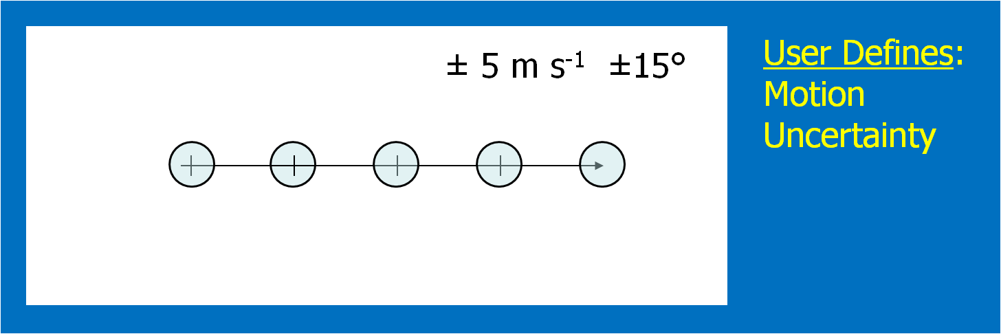
4.  Determine the uncertainty of the motion estimate.

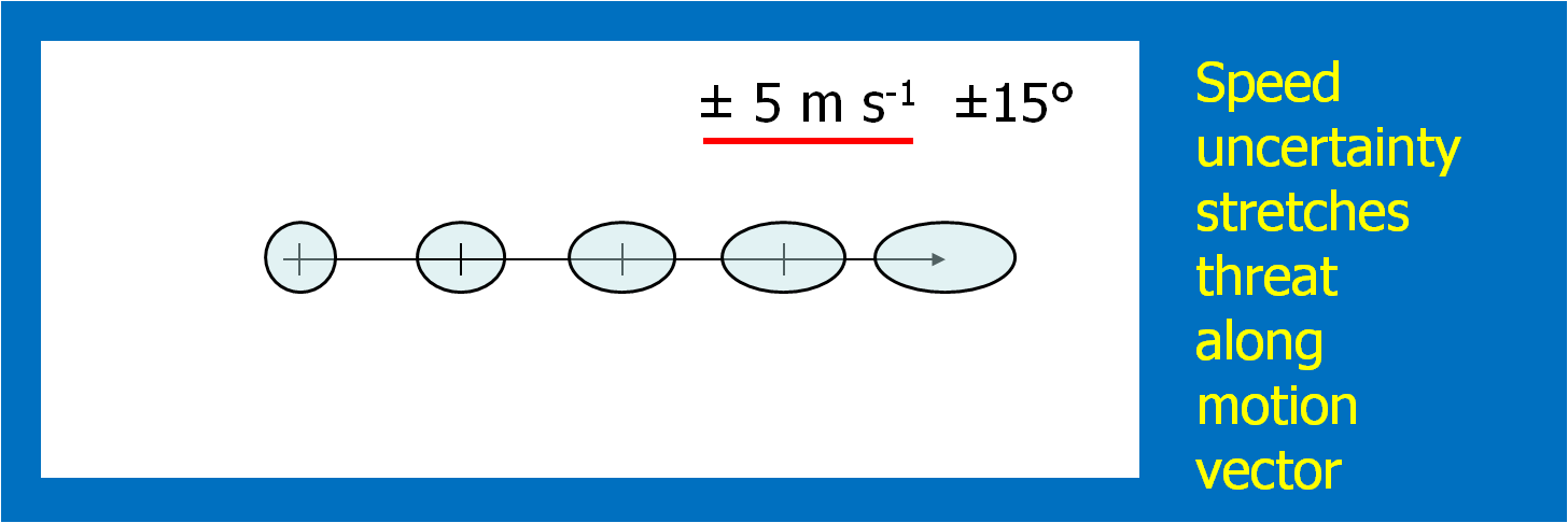
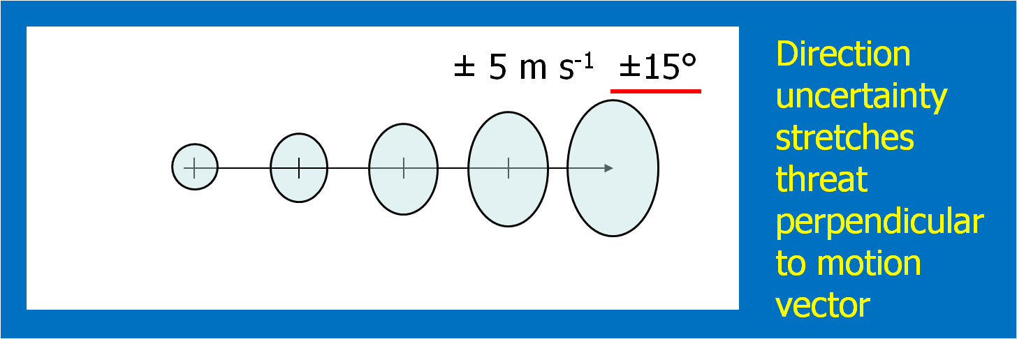
This could be approached in a number of different ways.  For the HWT experiments, the forecasters simply chose a range of symmetric speed and direction offsets.  For example, ±30° and ±5 kts.  Although we didn’t offer this choice during the 2007-8 HWT experiments, the offsets could be asymmetric (e.g., + 30°, -10°, +5 kts, -8 kts).  Fig. 6 shows an example offset for motion uncertainty.  Figs. 7 and 8 show how speed and direction uncertainty (respectively) affect the shape of the translating initial threat area in time.  Speed (direction) uncertainty stretches the initial threat area parallel (perpendicular) to the motion vector.

[More sophistication:  The motion uncertainty could come from a theoretical model of storm motion behavior, such as Bunkers’ storm motion estimate for right-turning supercell thunderstorms, or a statistical model such as the Thunderstorm Environment Strike Probability Algorithm (THESPA) technique (Dance et al., 2010; see their Eq. 1).]

Once the above four quantities have been chosen by the forecaster, we can then generate a downstream “swath” that will be affected by the translating threat area.  The swath is simply the total integration of all of the one-minute interval translating threat areas during the duration of the warning (Fig. 9).

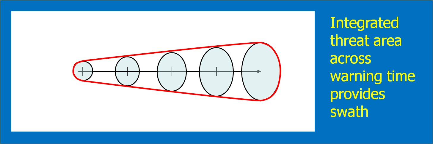
Here’s a better way to visualize the above static figure.  Figure 10 shows a loop of the translating threat area over the forecast interval.  The moving threat areas, integrated over the duration of the warning, providing the swath.

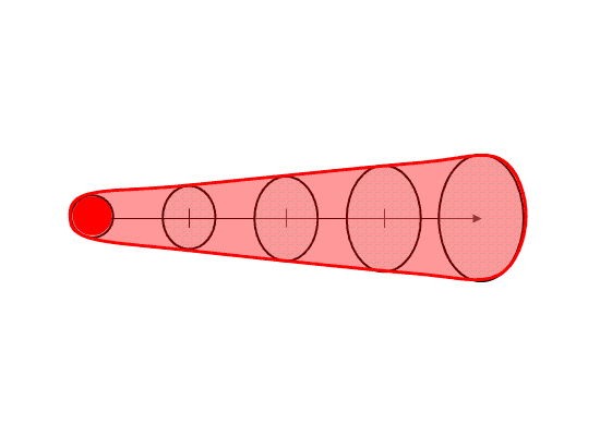
Note that the resulting “polygon” is exactly tied to the parameters of the warning as determined by the forecaster.  The resulting integrated polygon cannot (and should not) be editable.  The forecaster can only control the shape and position of the swath by changing the input parameters used to create the swath in order to ensure those values are always correlated with the integrated downstream swath.

The base digital grids that can be created in this process are the current threat area and the forecasted one minute translating threat areas out to the duration of the warning.  For our HWT experiments, we used a resolution of 1 km², which is the same resolution I employ within my geospatial warning verification methodology.  The forecasted one-minute interval threat grids can be used to create time-of-arrival and time-of-departure grids as well, which given the motion uncertainty information, can be expressed as a range of times (the range interval would decrease as the threat grew closer).  In addition, the integrated swath can also be saved as a digital grid.  The swath product can also be contoured to provide a series of lat/lon points that are analogous to today’s polygon warnings.  Metadata can also be added to the grids in the form of qualitative descriptions of the event, much like what is added to the WarnGen template output (e.g., “A TORNADO WITH DEBRIS WAS REPORTED AT HWY 9 AND JENKINS”).

The above four items were all that were required to create our digital hazard grids for the 2007-2008 HWT experiments.  How does this compare to the way forecasters issue warnings today using AWIPS WarnGen software?

• A current threat area is drawn, versus a point or line.
• Motion uncertainty is added.

That’s not much more than is currently input from the forecaster today.  Although it is slightly more information and workload, there are numerous benefits to this technique, which will be tackled in the next blog entry.

This concept isn’t the only way a current threat area can be forecasted.  In this methodology, the threat area expands based on forecaster input of motion uncertainty.  However, the uncertainty could also be based upon statistical analyses a la Dance et al. (2010; a Gaussian model).  Or, as we begin to approach the Warn-On-Forecast era, the extrapolated downstream threat areas might be enhanced by ensemble numerical model output to allow for discrete propagation, cell mergers, splits, growth, decay, and any other types of non-linear evolution of convective hazards.  The concepts presented here will form the framework for these future improvements.

Greg Stumpf, CIMMS and NWS/MDL