To consolidate the verification measures into one 2×2 contingency table and reconcile the area versus point issues, we place the forecast and observation data into the same coordinate system.  This is facilitated by using a gridded approach, with a spatial and temporal resolution fine enough to capture the detail of the observational data.  For the initial work that I am doing, I am using a grid resolution of 1 km² × 1 minute, which should be fine enough to capture the events with the smallest dimensions, namely tornado path width.  Tornado paths, and hail and wind swaths typically cover larger areas (and are not point or line events, as so depicted in Storm Data!).

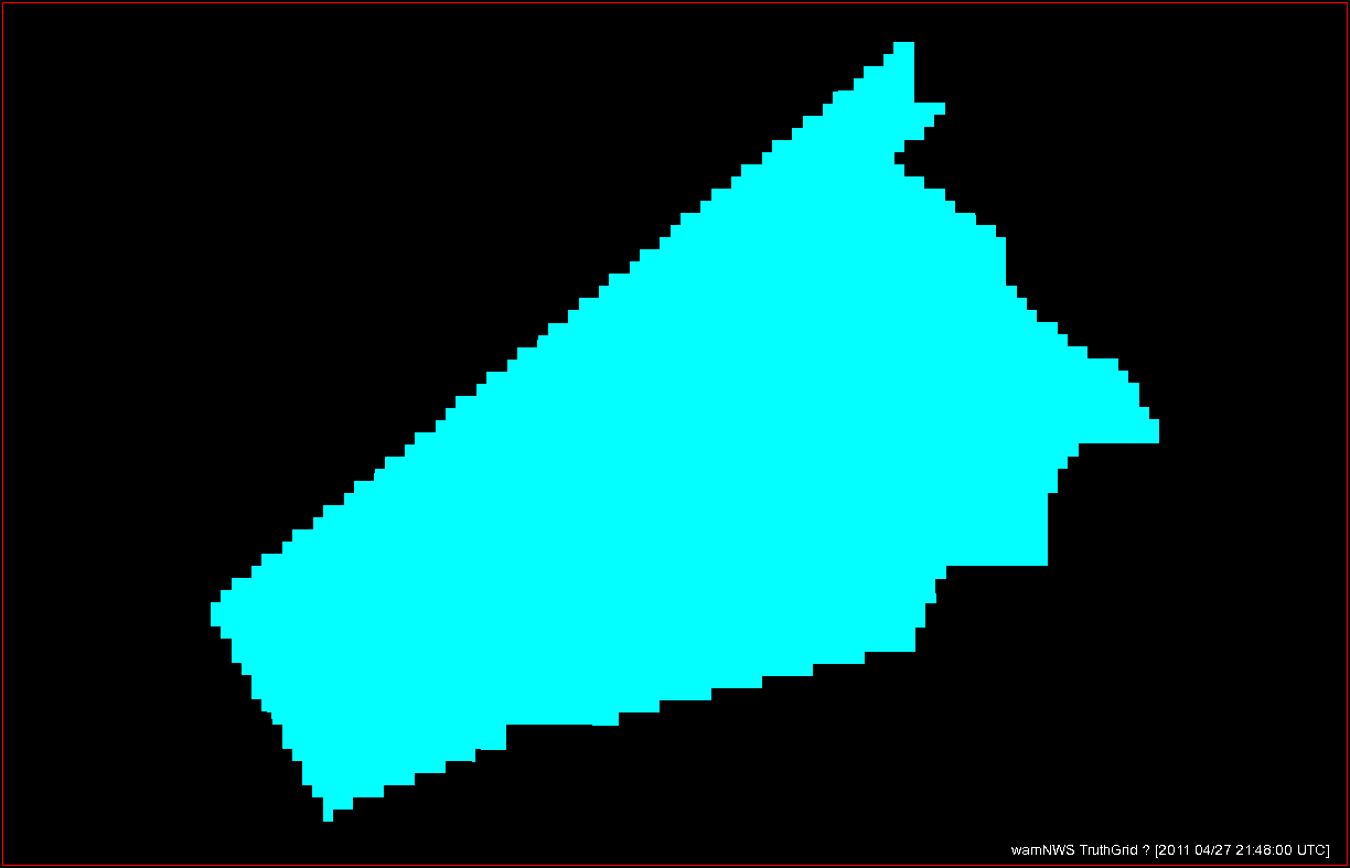
The forecast grid is created by digitizing the warning polygons (defined as a series of latitude/longitude pairs), and just turning the grid value to 1 if inside the polygon, and 0 if outside the polygon.  The grid has a 1 minute interval, so that warnings appear (disappear) on the grid the exact minute they are issued (canceled/expired).  Warnings are also “modified” before they are canceled/expired via use of Severe Weather Statements (SVS), and at those times, the warning polygon coordinates are changed.  These too are reflected in the minute-by-minute changes in the forecast grid.  Note that the forecast grid is currently represented as deterministic values of 0 and 1, but can easily be represented as any value between 0 and 1 to provide expressions of probability.  We won’t jump the gun on that and leave that subject to future blog entries.

The observation grids are created using either ground truth information, ground truth data augmented by human-determined locations using radar and other data as guidance, or radar proxies, or a combination of all of these.  As with the forecast grids, the values can be deterministic (only 0 and 1 – either under the hazard or not at that location and time) or fuzzy/probabilistic (e.g., location/time is not certain, or use of radar proxies which is also not certain).

For the purposes of my initial exercises, I will look at the verification of Tornado Warnings by tornado or radar-based mesocyclone observations for a specific storm case, the long-tracked tornadic supercell that affected Tuscaloosa and Birmingham Alabama on 27 April 2011 (hereafter, the “TCL storm”).  While it’s important to note that under some situations (the heavy workload of many storms or insufficient staffing levels), Tornado Warning polygons are sometimes drawn to encompass all of the storm threats, including the hail and wind threat along with the tornado threat, but we will ignore that for now and assume that the Tornado Warnings are verifying only tornado events.  Here’s a loop of the radar data, and the storm of interest ends up near the just crossing the AL-GA border on the upper right of the picture at the end of the loop.

To create my observation grid, I “truth” the tornado and mesocyclone centroid locations using radar data, radar algorithms, and damage survey reports.  I wrote a Java application that will convert the centroid truth data into netcdf grids at the 1 km² × 1 minute resolution.  This application first interpolates the centroid locations at even one minute intervals (e.g., 00:01:00, 00:02:00, being hh:mm:ss).  Then, for each one-minute centroid position, I create a “splat” that will “turn on” grid values within a certain distance of the centroid position (e.g., 5 km or 10 km).  The reason for the “splat” is to 1) account for small uncertainties in the timing and position of the centroids and 2) to allow for a buffer zone around which one may feel a location is “close enough” to the tornado to warrant a warning.  Finally, the “splat” consists of values between 0 and 1, with 1 being at the center of the splat, and values decreasing to 0 at the outer edge using an optional Cressman distance weighting function.  This provides “fuzziness” to the observation data, probabilistic observations in a sense.  The closer you are to the centroid location, the greater likelihood that the tornado was there.  This loop shows my tornado observation grid for the TCL storm.  Note that there were two tornadoes in Alabama from this storm (tornadoes #44 and #51 on this map provided by the NWS WFO Birmingham AL), hence the reason the truth “flashes out” in the middle of the loop.  Also note that we will not treat the tornado path with a straight path moving at a constant speed from its starting point to its ending point, as is done today with traditional NWS warning verification.

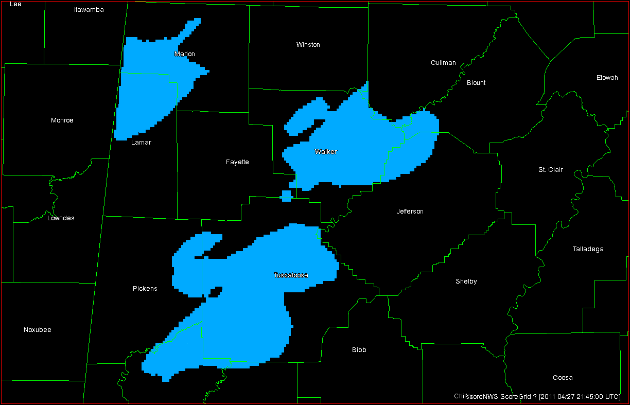
There is one more optional grid that is created to help define the observation data set.  When determining a CORRECT NULL (CN) forecast, if using every grid point outside of each warning polygon and each observation splat, the number of CN grid points would overwhelm all other grid points (tornadoes, and even tornado warnings are rare events), skewing the statistics (Marzban, 1998).  So we would like to limit the number of CN grid points to exclude those points where it is obvious that a warning should not be issued there – namely grid points which are away from thunderstorms.  Multiple-radar composite reflectivity (maximum reflectivity in the vertical column) is used for determining which grid points to use to calculate CN.  Optionally, one can choose the reflectivity value for the threshold of inside or outside a storm (I set this to 30 dBZ), and whether or not the reflectivity field should be smoothed using a median filter (I set this to true).  See here:

In the next blog entry, I’ll show what is done with all of these grid layers to compute the 2×2 table statistics.

ADDENDUM:  Up to this point, I haven’t explained my motivations for developing a geospatial warning verification technique.  In short, some of our Hazardous Weather Testbed (HWT) spring exercises with visiting NWS forecasters had them issuing experimental warnings using new and innovative experimental data sources and products during live storm events.  In order to determine if these innvoative data were helping the warning process, we compared the experimental warnings to a control set of warnings – those actually issued by the WFOs for the same storms on the same days.  We soon began to understand that the traditional warning verification techniques had some shortcomings, and didn’t completely depict the differences in skill between the two sets of warning forecasts.  In addition, the development of these techniques has me buried in Java source code within the Eclipse development environment – two major components of the AWIPS II infrastructure.  Finally, I hope to take information I’m learning from this exercise to start developing new methodologies for delivering severe convective hazard information and products within the framework of the current AWIPS II Hazard Services (HS) project, being designed to integrate several warning applications such as WarnGen and help pave the way for new techniques.  My hope is that my work pays off in several ways, from more robust methods to determine the goodness of our warnings from a meteorological and services perspective, to new methods of delivering hazard information, and finally to new software for the NWS warning forecaster, all in the name of furthering the NWS mission to protect lives and property.

REFERENCES:
Marzban, Caren, 1998: Scalar measures of performance in rare-event situations. Wea. Forecasting, 13, 753–763.

Greg Stumpf, CIMMS and NWS/MDL