Examining warning practices for QLCS tornadoes

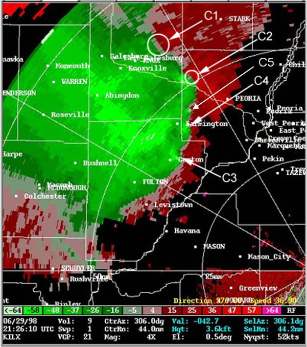
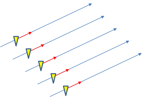
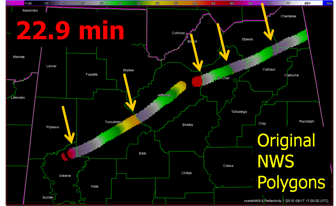
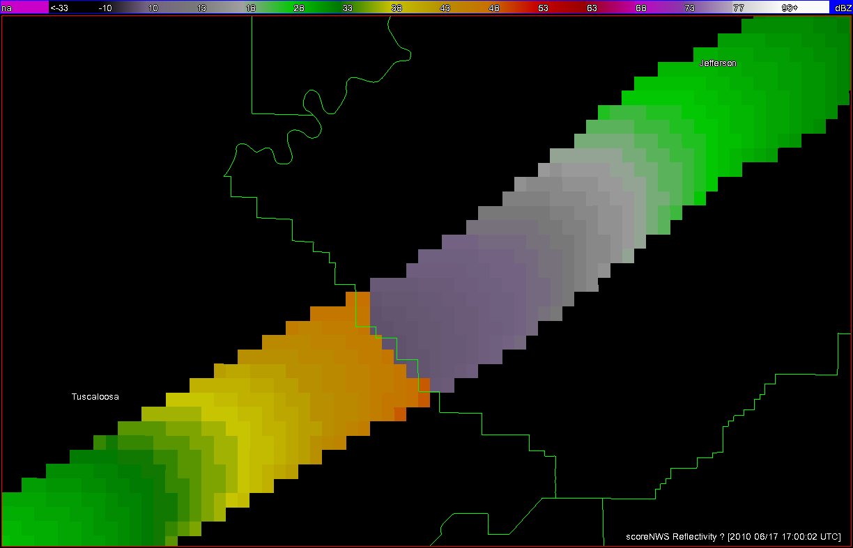
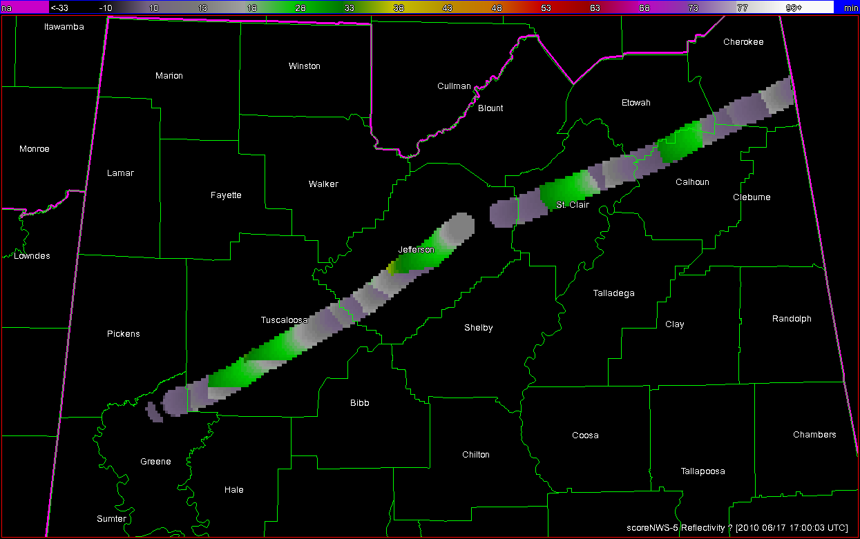
In the previous post, I examined the affects of warnings with more area on a single isolated long-tracked tornadic storm.  Now let’s look at a typical event that can comprise multiple tornadoes from independent mesocyclonic circulations, namely tornadoes along the leading edge of a Quasi-Linear Convective System (QCLS).  These are typically more challenging than supercell tornadoes to warn for because their existence, timing, and location can be more uncertain.  An example QLCS system with 5 vortices along the leading edge of the gust front is depicted here:

qlcs_example_annot

How are these situations warned for today?  Well, the strategies vary from WFO to WFO and from warning forecaster to warning forecaster.  In some instances, the large uncertainty of the event and sometimes high workload encourage forecasters to “cast a wide net” over the entire leading edge of the QLCS system with a single large and long Tornado Warning in hopes of not missing any tornado that might occur.  However, this may result and large areas falsely warned for considerable amounts of time. But if there are no tornadoes, it’s only one false alarm.  One of the pitfalls of our current warning verification system!

In other instances, forecasters might be more conservative and wait until a signature becomes apparent, and issue a smaller more-precise Tornado Warning for just that particular circulation.  However, in these instances, sometimes the warnings come late, resulting in either small lead times, or negative lead times with some or all of the portions of the tornadoes being missed.

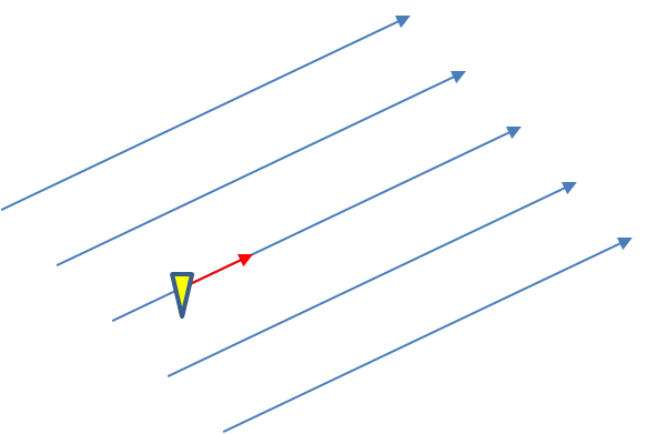
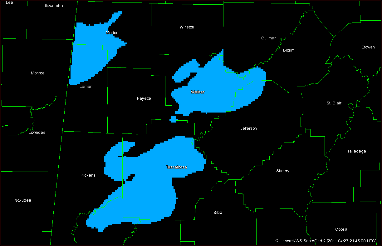
Let’s look at how both warning methodologies stack up when verified geospatially for a simulated QLCS event.  For the simulation, I created 5 parallel mesocyclone tracks that were 40 km apart, each starting and ending at the same time with a 60 minute duration and moving with the same motion vector (about 25 m/s from the southwest to the northeast).  As with the Tuscaloosa case, I used the mesocyclone centroid locations to determine the storm motion vector and position of the warning polygons, simulating a storm motion forecast with perfect skill using careful radar analysis.

I ran two warning methodologies.  In each case, the warnings expire after their intended duration and are never modified using the Severe Weather Statement (SVS) reduction method during their durations.  The warnings start at the same time in each scenario.

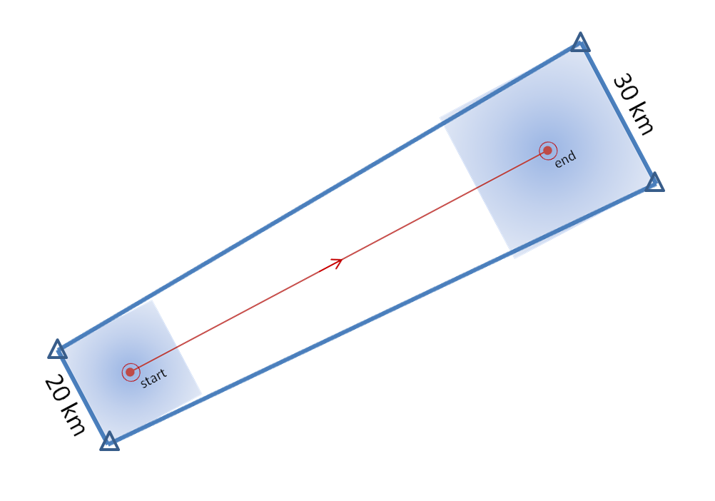
1warn: Issue one large warning using the default AWIPS WarnGen “line warning” polygon with an expiration time of 60 minutes.  To create the warning, a line is drawn from the centroid of the first mesocyclone to the centroid of the fifth mesocyclone at the beginning time of the warning.  This line is projected ahead 60 minutes using the storm motion vector.  A 10 km buffer is drawn surrounding the beginning line and a 15 km buffer is drawn around the ending line.  These are the same parameters used to create the default AWIPS WarnGen polygons for line warnings.  The far corners of each buffer are connected to create a four-sided polygon.  This is the “cast the wide net” scenario.

warngen240_line1

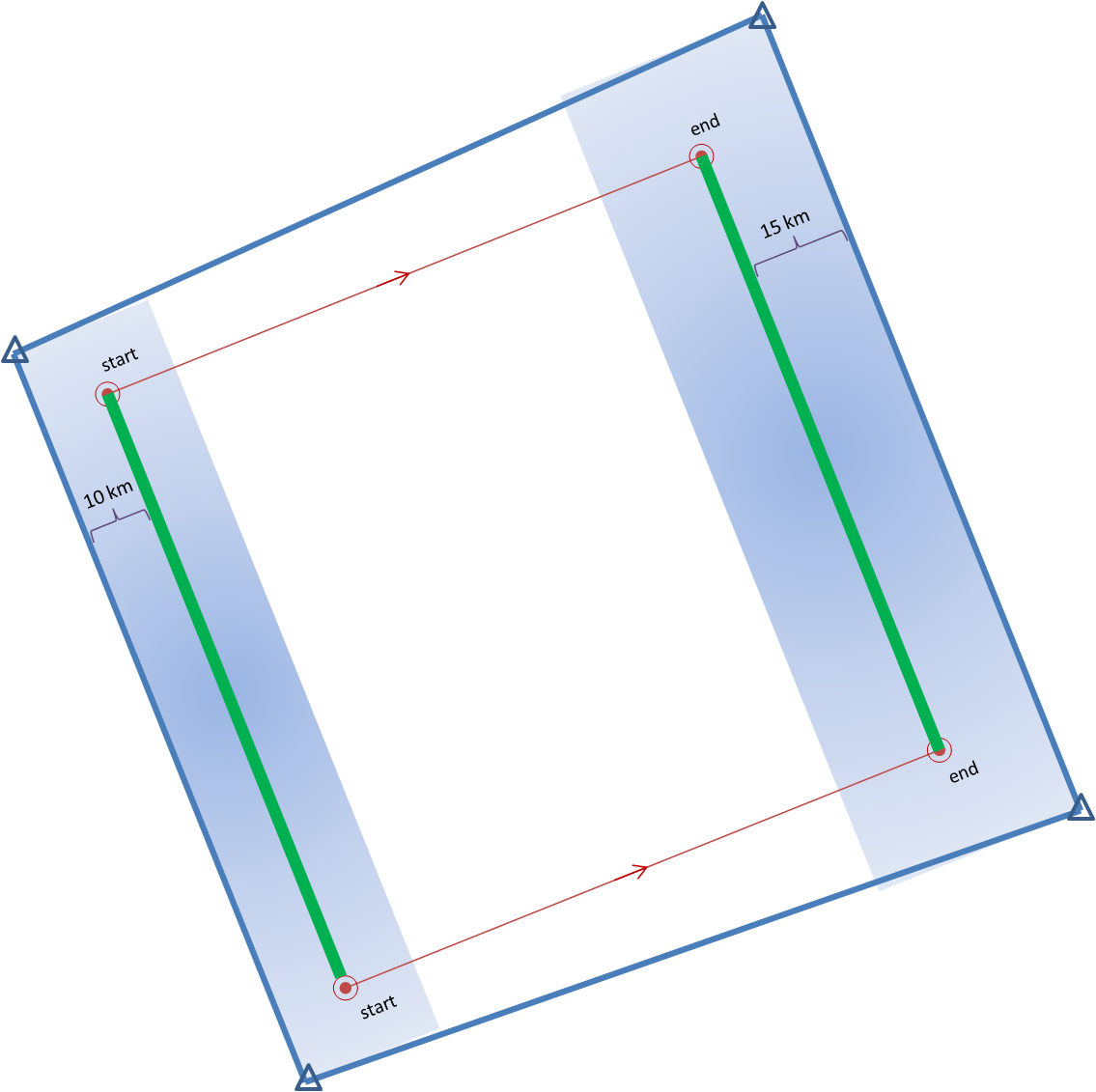
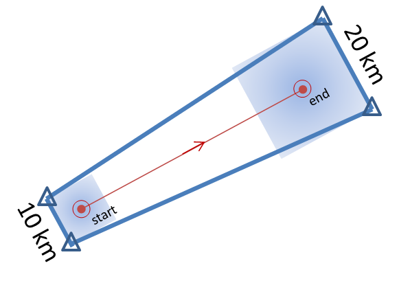
5warn: Issue five small warnings centered on each of the five individual mesocyclones.  The warning durations are set for 30 minutes (half the duration).  The warning polygon sizes are based on a 5 km buffer (10 km back edge) around the starting point of each warning, and a 10 km buffer (20 km front edge) around the projected ending point of each warning.  Note that these are smaller than the default buffer sizes, and are chosen so to simulate a more precise warning for what are typically short-lived tornadoes.  This is the “high precision” scenario.

warngen240-10-203

I then vary the outcome, the verification of the tornado events, in two ways:

1torn: Only one tornado: The middle (third) mesocyclone produces a tornado 10 minutes after the warnings were issued, lasting exactly 10 minutes.  The other four mesocyclones are non-tornadic.

1torn5

5torn: Five tornadoes:  All five mesocyclones produce a tornado 10 minutes after the warnings were issued, each lasting exactly 10 minutes.

5torn3

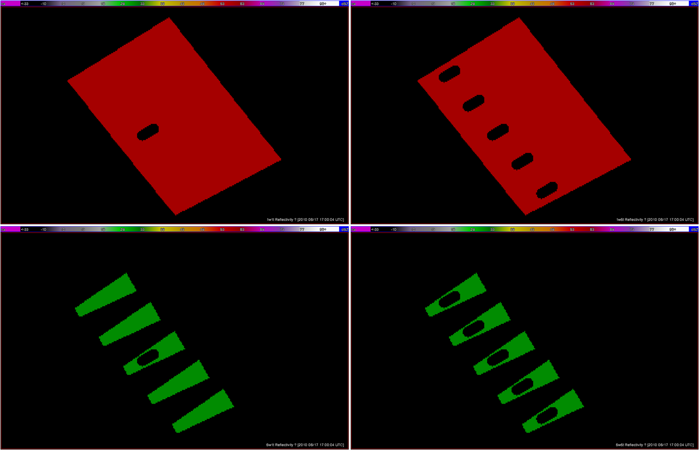
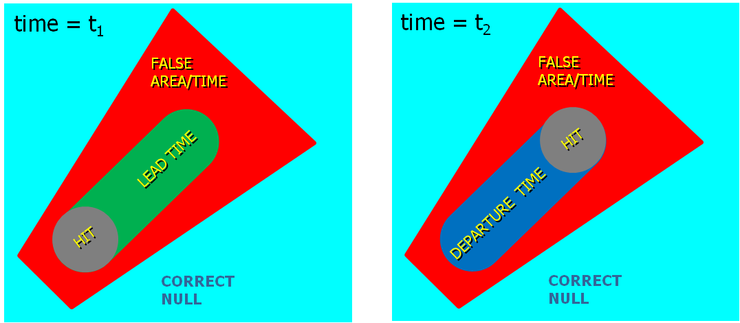
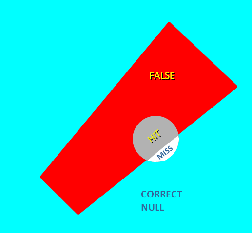
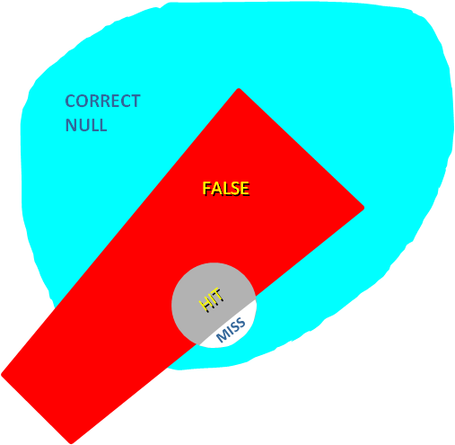
The four scenarios are illustrated in the figure below.  In each case, the dark regions inside the polygons represents the area swept out by the simulated tornadoes with a 5 km splat radius added.

qlcs_scenarios
Top left: Scenario 1warn-1torn; Top right: Scenario 1warn-5torn; Bottom left: Scenario 5warn-1torn; Bottom right: Scenario 5warn-5torn.

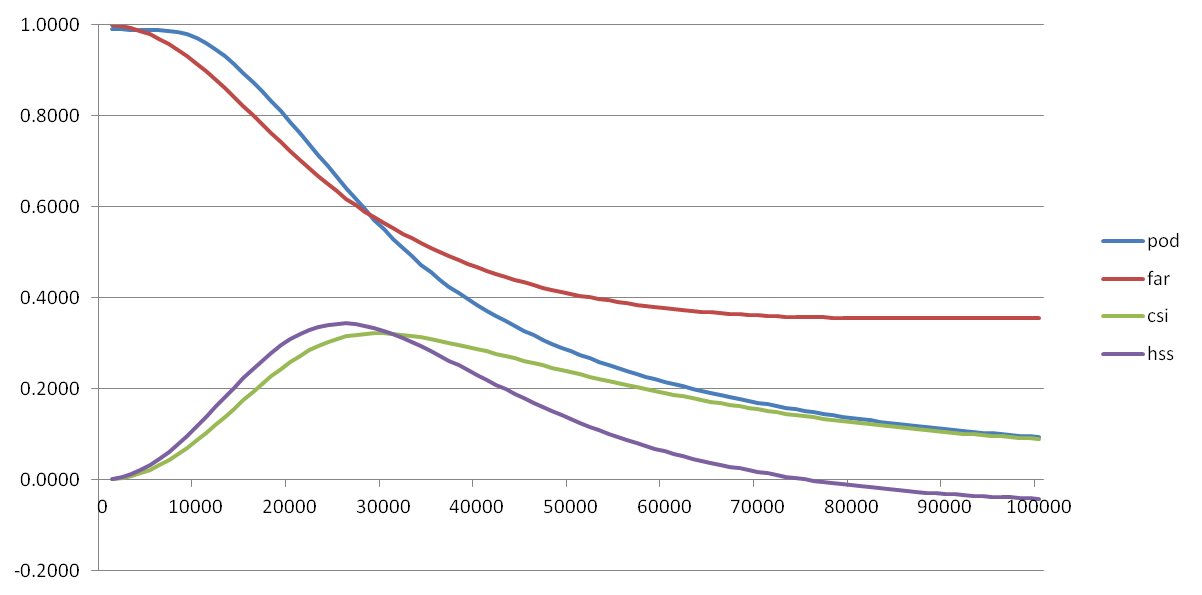
Let’s first consider the traditional warning verification stats for these four scenarios:

1warn-1torn:  POD 1.0, FAR 0.0, CSI 1.0

5warn-1torn:  POD 1.0, FAR 0.8, CSI 0.2

1warn-5torn:  POD 1.0, FAR 0.0, CSI 1.0

5warn-5torn:  POD 1.0, FAR 0.0, CSI 1.0

All but one of the scenarios results in prefect warning verification.  Scenario 5warn-1torn, 5 precise warnings and only one tornado, results in 4 “false alarms”.

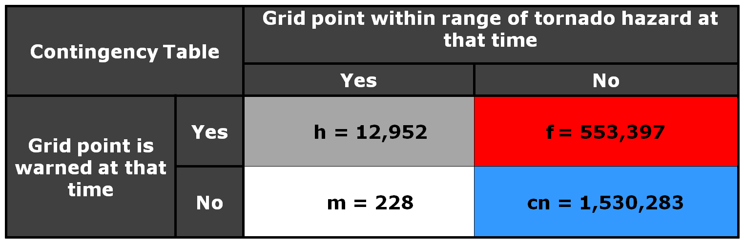
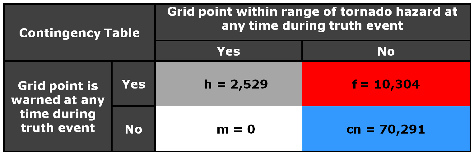
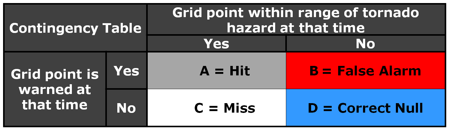
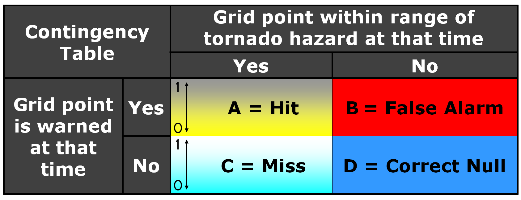
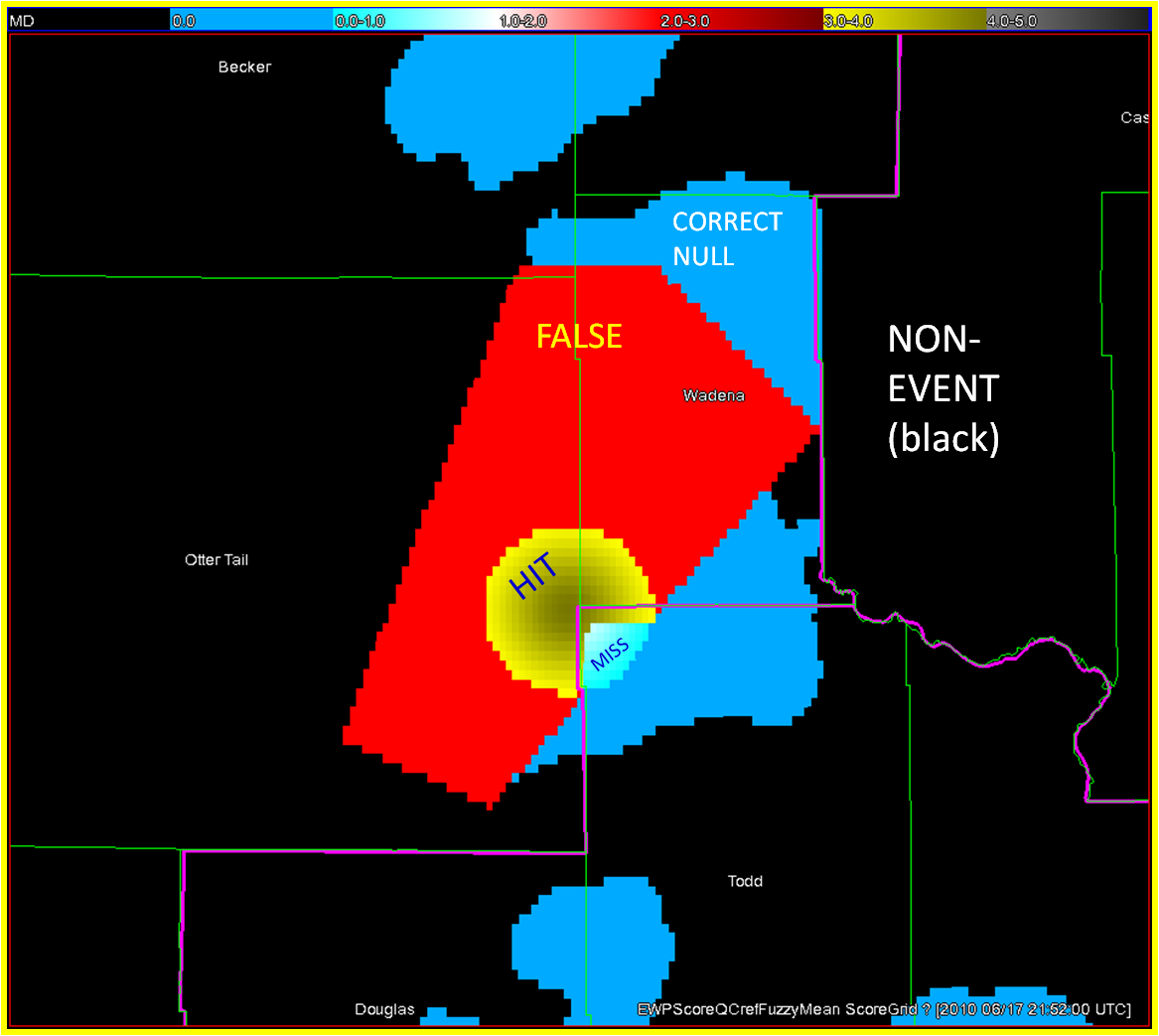
Now, how do these scores compare to using geospatial warning verification, where only one 2×2 table is used, and large false alarm area and times are considered poor performance?  Using the “grid point” verification method:

1warn-1torn:  POD 1.0000, FAR 0.9993, CSI 0.0007

5warn-1torn:  POD 1.0000, FAR 0.9942, CSI 0.0058

1warn-5torn:  POD 1.0000, FAR 0.9966, CSI 0.0034

5warn-5torn:  POD 1.0000, FAR 0.9709, CSI 0.0291

And using the “truth event” verification method:

1warn-1torn:  POD 1.0000, FAR 0.9894, CSI 0.0106

5warn-1torn:  POD 1.0000, FAR 0.9544, CSI 0.0456

1warn-5torn:  POD 1.0000, FAR 0.9471, CSI 0.0529

5warn-5torn:  POD 1.0000, FAR 0.7726, CSI 0.2274

Using each of these verification methods, the scenarios in which 5 separate precision warnings are issued have lower FARs and higher CSIs versus the large long-duration warning decisions for both the 1-tornado event and the 5-tornado events respectively.  In addition, there is the obvious difference in the scores when comparing the aggregate false alarm times for each scenario:

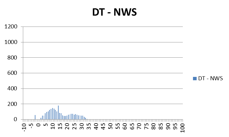
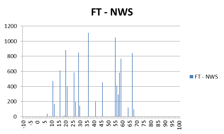
1warn-1torn:  FAT 1,101,120 km2-sec

5warn-1torn:  FAT 123,660 km2-sec

1warn-5torn:  FAT 1,054,020 km2-sec

5warn-5torn:  FAT 100,110 km2-sec

The 5 precision warnings result in total false alarm times that are about 1/10th of the large long-duration warnings.  So even given the case that 5 precision warnings are issued and only one tornado results, the time and area under false alarm is greatly reduced.

From a services standpoint, in the 5 precision warning case, there will be 5 separate alerts, 4 resulting in no tornado.  However, for the large warning scenario, there may only be “one alert”, but 10 times the area and time receiving the alert result in no tornado.  How do we deal with the issue that there will be more false alerts for the precision warning method?  We change the way we alert! More later…

ADDENDUM:  Jim LaDue of the NWS Warning Decision Training Branch (WDTB) wrote an excellent position paper describing why we should not adopt a practice to avoid issuing Tornado Warnings (and instead use Severe Thunderstorm Warnings) for the perceived notion that QLCS tornadoes are weak (EF0 and EF1).  Makes for excellent reading!

Greg Stumpf, CIMMS and NWS/MDL

Tags: None

The Benefits of Geospatial Warning Verification

Geospatial warning verification addresses both of the pitfalls explained in earlier blog entries by consolidating the verification measures into one 2×2 contingency table.  The verified hazards can be treated as two-dimensional areas, of which they are – storm hazards do not affect just points or lines!  We can include the correct null forecasts in the measures.  This method provides a more robust way to determine location-specific lead times as well as new metrics known as departure time and false time.  In addition, the method will reward spatial and temporal precision in warnings and penalize “casting a wider net” by measuring false alarm areas and false alarm times, which may contribute to a high false alarm perception by the public.

How might we measure the effect of the last issue addressed?  Let’s take our Tuscaloosa example and see what the effect of varying the warning size and duration has on our verification numbers.  I will only present a few test cases here, because I want to eventually explore this further with a different storm case that isn’t comprised of a single long-tracked isolated storm.

I developed a method which will take my truthed mesocyclone centroid locations and use them to compute the storm motion vector as specific warning decision points along the storm track.  Starting from the initial warning decision point from the BMX WFO on the TCL storm (2038 UTC 27 April 2011), I created warning polygons using the default AWIPS WarnGen polygon shape parameters.  Namely, the current threat point is projected to its final position using the motion vector and a prescribed warning duration.  A 10 km buffer is drawn around the starting threat point resulting in the back edge of the warning being 20km.  A 15 km buffer is drawn around the ending threat point resulting in the back edge of the warning being 30km.  The far corners of each box are then connected to create the trapezoid shape of the default warning polygon.

warngen2403

I used a 60-minute warning duration since the NWS warnings were also about 60 minutes in duration for the TCL storm.  I have a re-warning interval of 60 minutes, so that a new warning polygon is issued as the hazard location is nearing the downstream end of the current warning polygon.  Because of the buffer around the projected ending point of the threat, each successive warning will have some overlap with the previous warning, which is considered a best warning practice.  None of the warnings will be edited for shape based on any county border, because we want to test the effect of warning size and duration without any other factors influencing the warning area.  A loop of the warning polygons with the mesocyclone path overlaid:

warn-6060x10-loop1

Here is the 2×2 table using a 5 km radius of influence (“splat”) around the one-minute tornado observations, I am not applying the Cressman distance weighting to the truth splats, and I’m using the composite reflectivity filtering for the correct nulls:

ctable_tcl_004

And the grid point method scores are:

POD = 0.9827

FAR = 0.9771

CSI = 0.0229

The FAR and CSI are slightly better than the NWS warnings.  However, I’m not trying to compare this method to the actual warnings, but rather as a start to determine the effect of larger and longer warning polygons.  So, let’s try that now.  Instead of using starting and ending box sizes of 20 and 30 km respectively for our default WarnGen polygon, let’s cast a wider net and quadruple that to 80 and 120 km.  The polygon loop would look like this:

warn-6060x40-loop

And the 2×2 table and scores like this:

ctable_tcl_0051

POD =1.0000

FAR = 0.9962

CSI =0.0038

What was the effect of the larger longer polygons?  Well first, there were no missed grid points, and the POD = 1.  But the number of false alarm grid points increased by a factor of about 7, and thus the FAR went up and the CSI went down.  Recall that the number of false alarm grid points represents the number of 1 km2 grid points accumulated for each minute of data, so the false alarm area and time are much larger, even though these warnings verified perfectly.

So let’s take this in the opposite direction and make our warning polygons smaller.  We’ll use starting and ending box sizes of 6 and 10 km respectively.  The loop:

warn-6060x3-loop1

and the numbers:

ctable_tcl_0061

POD = 0.6668

FAR = 0.9422

CSI =0.0561

We’ve significantly reduced the false alarm area, but we also negatively affected the POD.  About 1/3 of the tornado grid points were missed because the warnings were too small.

Now, let’s run the “Truth Event” statistics on all three scenarios:

3 km:  pod 0.6390, far 0.3041, csi 0.4995, hss 0.6563, lt 32.8, dt 27.4, ft 61.8

10 km: pod 0.9968, far 0.6780, csi 0.3217, hss 0.4619, lt 39.0, dt 32.1, ft 71.3

40 km:  pod 1.0000, far 0.9164, csi 0.0836, hss 0.1015, lt 73.2, dt 46.7, ft 114.6

The 3 km warnings have the best CSI and HSS.  This appears that the geospatial verification scheme is rewarding more precise polygons.  But there is a problem…there is also a pretty low POD, which means that portions of the tornadoes are not being warned.  That’s not good, and reflective of the Doswell “asymmetric penalty function” where forecasters are harmed more by missed tornadoes than false alarms.  Why is this so?  Because our warnings are being issued for 60 minute durations and 60-minute re-warning intervals.  That means for these narrow warnings, if the storm motion deviates after the warning is issued, then there is no chance to re-adjust the warning to account for the storm motion changes.  Hence, a larger warning would capture these changes.

One might wonder – how can we balance precision and high POD?  I will treat this issue in a later blog, but for now, the next entry will continue to look at the issues of casting a wider net as it pertains to a very hot topic right now – how to warn for Quasi-Linear Convective System (QLCS) tornadoes.

Greg Stumpf, CIMMS and NWS/MDL


Tags: None

Creating Verification Numbers Part 5: Distribution of “Truth Event” statistics

We can dissect the stats a little more.  First, let’s look at the overall distribution of LEAD TIME (LT), DEPARTURE TIME (DT), and FALSE TIME (FT) for all truth events to get an idea about the range of values.  The following histograms depict the distribution of values for each grid point.  These graphs show a lot more information than the average values for each presented in the last blog post.

lt_nws

For LEAD TIME (LT), you can see that for some of the grid points, there were some negative lead times, and a fair number of grid points with lead times below 10 minutes.  Also note the few grid values above 55 minutes.  These were caused by the start of the two tornadoes forming at the very far ranges of the warnings covering their storms.  Looking at the lead times for just the starting time of those two tornadoes, the numbers end up being fantastic:  65 minutes and 57 minutes respectively, according to the NWS Verification statistics.  But as we are showing here, it is important to consider the lead time between warning issuance and tornado impact at each specific location along the path of the tornado, and for some of those, the numbers don’t reflect as good a level of success as those two numbers above.   We will explore this further in just a second.

dt_nws

For DEPARTURE TIME (DT), we can see that warnings were cleared out anywhere from 0 minutes to as much as about 35 minutes after the threats had passed.  Should warnings remain in effect for so long?  The clearing of warning polygons via Severe Weather Statements (SVS) serves this purpose, but it is a manual process that does not have a standard protocol from WFO to WFO, and sometimes isn’t done when workload is too demanding.  Also note a few data points in the negative area – these are warnings that were cleared too early – the threat was still affecting those locations.  However, recall that our threat locations have a 5 km splat radius around them; these data points come from the very back end of some of these splats at the early stages of the first tornado.

ft_nws

The FALSE TIME (FT) distribution looks much different than the other two, it is more “disjointed”.  The main reason for this is because these values are based on the warnings and not the one-minute updating tornado threat locations, so there will be discontinuities associated with each change in the warning polygons, which comes about every 15 minutes as new warnings are issued or current warnings are reduced in size via SVS.  But note that there are some locations that are falsely warned for over 60 minutes!  This is even though the storm-based polygon warnings were technically not false alarms according to traditional NWS warning verification methods.

Because our data are geospatial, we have the luxury of looking at the geospatial distribution of the LT, DT, and FT values on a map!  Let’s start with the LEAD TIME (LT) graphic:

LT-NWS-map

What you are seeing here are the LEAD TIME values at specific locations along the path of the two tornadoes, with the 5 km “splat” buffer added (no values are recorded outside the path of the threat).  Pay particular attention to the five yellow arrows.  We’ll zoom in on one of them:

lt_discontinuity

What we are seeing here is a discontinuity in LEAD TIME at this location of the tornado path.  Values at the far end of Tuscaloosa County are 47 minutes, while at adjacent grid points downstream in Jefferson County, the lead times on the tornado path were only 3 minutes.  These inequitablies are the result of warnings being issued one after the other, with the threats nearing the end of one warning polygon before the next downstream polygon is issued.  This is evident in the NWS polygon warning loop I showed in a previous blog entry.  There are five of these discontinuities in the path of both tornadoes from this storm.  These five discontinuities represent the downstream end of the first five polygons that were issued by the NWS on this storm (the 6th polygon warning expired on the AL-GA state line, so the discontinuity is not seen because I didn’t include the grid points within Georgia).  The same five discontinuities are also seen if we plot the one-minute tornado segment lead times available from the NWS Verification database:

TCL_lead time

The graphical DEPARTURE TIME map:

warnNWS_DT

More discontinuities are seen here because in addition to the new warnings being issued, there were the numerous removals of the back ends of the polygons via the SVSs.

This final graphic depicts the FALSE TIME (FT) per grid locations.  Values only exist where warning polygons were in effect outside the path of the tornado plus the 5km splat.

warnNWS_FT

There is quite a bit of area that is falsely warned (assuming the 5 km buffer around the tornado), and many of these areas are warned for over 60 minutes.  Note each warning polygon and subsequent SVS edit becomes evident on this graphic.  Note too that for the second tornado the warning polygons are placed with the tornado path to the right of center (as viewed toward the storm motion direction), which indicates that the warning forecaster probably started using the Tornado Warnings to cover the entire severe threat (wind, hail) and not just the tornado threat.

Next up, a summary of the benefits of geospatial warning verification, and then an exercise illustrating the second pitfall of “casting the wider net”.

Greg Stumpf, CIMMS and NWS/MDL

Tags: None

Creating Verification Numbers Part 4: “Truth Event” scores for one event

Now that I’ve outlined how “Truth Event” scoring is accomplished, how well did it do for the Tuscaloosa-Birmingham long-track supercell event from 27 April 2011?  Recall that a “truth event” is defined as a continuous time period a specific grid point is under a warning(s) and/or a tornado observation(s) surrounded by at least one minute of neither.  What are the various quantities that can be calculated for each truth event?  Beginning with these values:

twarningBegins = time that the warning begins

twarningEnds= time that the warning ends

tobsBegins = time that the observation begins

tobsEnds= time that the observation ends

Given these various times, the following time measures can be calculated for each truth event:

LEAD TIME (lt): tobsBegins twarningBegins [HIT events only]
DEPARTURE TIME (dt): twarningEnds tobsEnds [HIT events only]
FALSE TIME (ft): twarningEnds – twarningBegins [FALSE events only]

Then we can take all the truth events and add up the number of HIT EVENTS, FALSE EVENTS, MISS EVENTS, and CORRECT NULL EVENTS, and put them into our 2×2 contingency table.  As before, I am using a 5 km radius of influence (“splat”) around the one-minute tornado observations, not applying the Cressman distance weighting to the truth splats, and I’m using the composite reflectivity filtering for the correct nulls:

ctable_tcl_0031

First note that the raw numbers in this 2×2 table are much smaller than those from the “Grid Point” method of scoring.  Recall that the first scoring method counted each grid point as a single data point at each one minute time step.  For the “Truth Event” scoring, multiple grid values at multiple time steps are combined into a single truth event.  Also note that there are no truth events categorized as a MISS EVENT.  That means that every grid point within a 5km radius of the two tornado paths were at one period during the event covered by a warning.  Remember that there was a 2-minute gap in the warnings when the tornado was southwest of Tuscaloosa.  However, since those grid points were eventually warned, they were considered HIT EVENTs, but their lead time ends up being negative.

Here are the various numbers for the truth events:

POD = 1.0000

FAR = 0.8029

CSI = 0.1971

HSS = 0.2933

When comparing these to the grid point style of scoring, there seems to be improvement in all areas.  But note that these are based the fact that each truth event is considered equal, no matter how long that event was.  A one-minute false alarm and a 60-minute false alarm are each counted as one false alarm.  Sounds like one of our original traditional warning verification pitfalls.  But we have information about the time history of each truth event, and can extract even more information out of them.  This is where the time measures come in.  Computing the average of the various time measures for all grid points:

Average Lead Time (lt) = 22.9 minutes

Average Departure Time (dt) = 15.2 minutes

Average False Time (ft) = 39.8 minutes

Now we can get a more complete picture of how well the warnings did for all of the specific geographic locations.  From the NWS Warning verification data base, the average lead time for all the one-minute segments for both tornadoes with this storm is 22.1 minutes.  This is very close to that number above, because our gridded verification data also has one minute intervals, but we are also counting grid points within 5 km of the tornado at each minute, which increases the number of data points by about 80x.  Also remember that the ground truth I used was more spatially-precise than a straight line connecting the start and end positions of the tornado, and more temporally-precise in that the one-minute locations are not based on an equal division of the straight path between end points.

Regarding DEPARTURE TIME, this is new metric that can be calculated.  In this case, each grid point affected by the 5km tornado “splat” remains, on average, under a Tornado Warning for an extra 15.2 minutes even though the tornado threat has already cleared.

And with FALSE TIME, we can now extract information back out of the truth event numbers to tell us that our warnings may be too large or too long.  In this case, of the grid points warned but not affected by the tornado, on average, these grid points were “over-warned” by 39.8 minutes.  And to get a representation of the approximate False Alarm Area, 10,304 square kilometers of ground were falsely warned for at least one minute.

In the next blog post, we will dissect the truth event statistics a little more, looking at various numerical and geospatial distributions.

Greg Stumpf, CIMMS and NWS/MDL

Tags: None

Creating Verification Numbers Part 3: The “Truth Event” method

There are several drawbacks of the “Grid Point” method that we need to address.  First, how do we account for grid points that are downstream of an observation event that are expected to be covered by that event on a future grid?  Should these be considered false alarm grid points?  And how about grid points that are behind an event that has already passed that location?  Second, the previous method has no easy way to compute lead times for specific grid point locations.  To address these issues, we’ve developed the second method of geospatial warning verification, namely the “Truth Event” method.

A “truth event” is defined as a continuous time period a grid point is under a warning(s) and/or a tornado observation(s) surrounded by at least one minute of neither:

FALSE EVENT: If grid point remains in “false” condition throughout event (only forecast grid becomes “> 0”).  These grid points do not receive an observation of a hazard, but were warned.

MISS EVENT: If grid point remains in “miss condition” throughout event (only observation grid becomes “> 0”).  These grid points were not warned, but received an observation of a hazard.

HIT EVENT: If grid point experiences a “hit condition” for at least 1 minute during event (fcst and obs are both “> 0”).  These grid points were warned AND received an observation of a hazard.

“Hit Events” can then be comprised of several different scenarios.  The most common scenario would be this: 1) a warning is issued for a particular grid point, 2) a hazard observation impacts that grid point after warning issuance, 3) the hazard observation leaves the grid point while the warning remains in effect, and 4) the warning expires or is cancelled for that grid point.  For these scenarios, the grid points will be in FALSE condition prior to and after the hazard passes over that location.  For the Truth Event method, these conditions are not considered FALSE, but instead are depicted as “LEAD TIME” and “DEPARTURE TIME”, respectively.  To see this graphically:

leadtime

Hopefully this makes some sense.  What you are seeing above are two snapshots of the grids at two times, t1 and t2. Let’s say we were to look at the “truth event” for one of the grid points in the figure, perhaps one that is right near the letter “L” in “LEAD TIME” on the t1 image on the left:

truth-event-011

The truth event is defined by starting and ending time of the warning.  Since the warning was issued prior to the observation impacting the grid point, you get positive LEAD TIME.  This verification method rewards larger lead time.  Although there is some discussion about how much lead time might be “too much”, we will table that discussion for now, and revisit it on a later blog entry.  Note that if an observation impacts a grid point prior to a warning, then we can measure negative LEAD TIME, which is considered not good.  But if an observation impacts a grid point that is never warned, then no LEAD TIME is recorded.  This differs from the current NWS verification method, which records a zero (0) LEAD TIME for missed events.

This verification method also allows us to analyze a new kind of metric which we will call DEPARTURE TIME.  This is the amount of time that a grid point remains under a warning after the threat has already passed by.  Ideally, the DEPARTURE TIME should be zero – the warning is canceled or expires immediately just after the threat has passed.  Positive DEPARTURE TIME, as shown in the above examples, is chosen to represent the condition when the warning remains in effect after the threat has passed (a FALSE condition, in a sense).  Negative DEPARTURE TIME is chosen to represent the condition when the warning has expired before the threat has passed (a MISS condition, in a sense).  This truth event scenario depicts negative LEAD TIME and negative DEPARTURE TIME, the warning was late plus the warning was canceled too early:

truth-event-02

We can also analyze a third kind of metric which we will call FALSE ALARM TIME.  This is for truth events that remain in FALSE EVENT condition through their time period.  The time line of that kind of truth event is shown here:

false-event-01

More soon…

Greg Stumpf, CIMMS and NWS/MDL

Tags: None

Creating Verification Numbers Part 2: Grid point scores for one event

In order to illustrate the kinds of measures we can get from this method of warning verification, let’s first look at a single storm event.  The chosen storm will be the 27 April 2011 long-tracked tornadic supercell that impacted Tuscaloosa and Birmingham, Alabama.  This was a well-warned storm from the perspective of traditional NWS verification.

It helps to first look at the official NWS verification statistics for this event.  The storm produced two verified tornadoes along its path within the Birmingham (BMX) County Warning Area (CWA).  The BMX WFO issued 6 different Tornado Warnings covering this storm over 4 hours and 22 minutes (20:38 UCT 27 April – 01:00 UTC 28 April), from the AL-MS border northeastward to the AL-GA border.  Here’s a loop showing the NWS warnings in cyan, and the path of the mesocyclone centroid overlaid.  In the loop, it may appear that more than 6 different warning polygons were issued.  Instead, you are seeing warning polygons being reduced in size via their follow-up Severe Weather Statements (SVS) in which the forecasters manually remove warning areas behind the threats.

warn-NWS-loop-fast1

All 6 warnings verified in the traditional sense – each contained a report of a tornado, and both tornadoes were warned.  There were no misses and no false alarms.  Thus, the Probability Of Detection = 1.0, the False Alarm Ratio = 0.0, and the Critical Success Index = 1.0.  Boiling it down further, if we use the NWS Performance Management site, we can also determine how many of the 1-minute segments of each tornado were warned.  It turns out that not every one segment was warned, as there was a 2-minute gap between two of the warnings (while the storm was southwest of Tuscaloosa – you can see the warning flash off in the above loop).  So there were 184 minutes warned out of the total of 186 minutes of total tornado time, giving a Percent Event Warned (PEW) of 0.99.  Still, these numbers are very respectable.

Now, what do the geospatial verification statistics tell us?  We’ll start by looking at the statistics using a 5 km radius of influence (“splat”) around the one-minute tornado observations.  For this 2×2 table, I am not applying the Cressman distance weighting to the truth splats, and I’m using the composite reflectivity filtering for the correct nulls:

ctable_tcl_0011

Remember that the values represent the count of 1 km2 x 1 minute grid points that met one of the 4 conditions in the 2×2 table. If we compute the POD, FAR, and CSI, we get:

POD = 0.9885
FAR = 0.9915
CSI = 0.0085

The POD looks very similar to the PEW computed using the NWS method. But the FAR and CSI are much much different. The FAR is huge, and thus the CSI is really small! What this tells us that for each one minute interval of the 4 hours and 22 minutes of warning for this event, over 99% of the grid points within the warning polygons were not within 5 km of the tornado at each one minute interval, accumulated. Is this a fair way to look at things? It is one way to measure how much area and time of a warning is considered false.  The big question is this – what would be considered an acceptable value of accumulated false alarm area and time for our warnings?  Given the uncertainties of weather forecasting/warning, and the limitations of the remote sensors (radar) to detect tornadic circulations, I don’t think we can ever expect perfection – that the warnings perfectly match the paths of the hazards.  But this should be a method for determining if our warnings are being issued too large and too long in order to “cast a wide net”.

One way to analyze this is to vary the size of the “splat” radius of influence around each one-minute tornado observation.  For example, if we were to create the above 2×2 table and stats using a 10 km “splat” size (instead of 5 km), the numbers would look like this:

ctable_tcl_0021

POD = 0.9702
FAR = 0.9141
CSI = 0.0857

Note that the FAR is starting to go down, from 0.99 to 0.91.  But the POD is also starting to lower slightly.  Why, because now we’re requiring that the warnings cover the entire 10 km radius around each one minute tornado “splat”, so more of the observation area is starting to get missed by warnings.

Is 5 or 10 km the correct buffer zone around the tornadoes?  Or is it some other value?  Let’s look at the variation in POD, FAR, CSI, and the Heidke Skill Score (HSS; uses the CORRECT NULL numbers) across varying values of splat size, from 1 km to 100 km at 1 km intervals (the x-axis shows meters on the graph):

podfarcsihss_0011

This graph might imply that, based on maximizing our combined accuracy measures of CSI and HSS, that the optimal “splat” radius should be around 25-30 km.  Instead, this probably shows that the average width of the warnings issued that day were about 25-30km wide, and if given a requirement to warn within 25-30 km of the tornadoes, the NWS warnings would be considered good.  So we’re still left with the question – what is the optimal buffer to use around the tornado reports?  This is probably a question better answered via social science.  And, given that number, what is an acceptable false alarm area/time for the warning polygons?  In other words, what would our users allow as an acceptable buffer, and can meteorologists do a decent job communicating that this buffer is needed to account for various uncertainties?

What about grid locations away from the tornado but will be impacted at a later time?  They are downstream of the tornado headed toward them. Should they be counted toward the false alarm numbers? My answer is no and yes. I will tackle the ‘no’ now, and the ‘yes’ answer will come much later in this blog.

Greg Stumpf, CIMMS and NWS/MDL

Tags: None

Creating Verification Numbers Part 1: The “Grid Point” Method

Now that we have our one-minute forecast grids (warnings), our one-minute observation grids (“splatted” tornado locations), and our additional third grid to filter for CORRECT NULL forecasts (median filtered composite reflectivity), let’s combine them to fill our single 2×2 contingency table, shown here:

ctable_not-fuzzy1

At each one-minute forecast interval, we can create these grid point values:

HIT:  The grid point is warned AND the grid point is within the splat range of a tornado.

MISS:  The grid point is not warned AND the grid point is within the splat range of a tornado

FALSE:  The grid point is warned AND the grid point is outside the splat range of any tornado.

CORRECT NULL:  All other grid points (outside warnings and outside tornado observations).

Viewing this graphically (the cyan CORRECT NULL area is supposed to fill the entire domain in this figure):

score_grid

If we want to limit the number of grid points counted as CORRECT NULL, we can incorporate the third composite reflectivity grid:

CORRECT NULL:  The grid point is not warned AND the grid point is outside the splat range of any tornado AND the grid point has a composite reflectivity value > 30 dBZ.

NON-EVENT:  The grid point is not warned AND the grid point is outside the splat range of any tornado AND the grid point has a composite reflectivity value < 30 dBZ.

Viewing this graphically (the cyan CORRECT NULL area is only within the “storm area” in this version):

score_grid_cn

If we choose to score using a fuzzy representation of the observation based on the Cressman distance weighting scheme, the 2×2 table might look like this:

ctable_fuzzy1

And the scoring categories become:

HIT:  A value between 0 and 1 based on the Cressman weight value.  At the center of the observation splat, this is 1.  At the farther range of the splat, this is 0.  The value is between 0 and 1 for locations between these two ranges.

MISS:  A value between 0 and 1 based on the Cressman weight value.  At the center of the observation splat, this is 1.  At the farther range of the splat, this is 0.

FALSE:  1 – HIT.  This value is 1 when grid is completely outside the splat range of any tornado observation.  Within the splat range of a tornado observation, FALSE + HIT = 1.

CORRECT NULL:  1 – MISS.  This value is 1 when grid is completely outside the splat range of any tornado observation.  Note that the grid point must also have a composite reflectivity value > 30 dBZ. Within the splat range of a tornado observation, CORRECT NULL + MISS = 1.

NON-EVENT:  The grid point is not warned AND the grid point is outside the splat range of any tornado AND the grid point has a composite reflectivity value < 30 dBZ.

Viewing this graphically (using a different, but an actual event – 17 June 2010 Wadena, MN):

score_grid_cn_fuzzy

We can then run our 2×2 statistics on each one-minute interval during a warned tornado event and accumulate them for the entire event.  The results can be somewhat surprising, and they will need some interpretation.  That will be the subject of the next blog entry.

Greg Stumpf, CIMMS and NWS/MDL

Tags: None

Geospatial Verification Technique: Getting on the Grid

To consolidate the verification measures into one 2×2 contingency table and reconcile the area versus point issues, we place the forecast and observation data into the same coordinate system.  This is facilitated by using a gridded approach, with a spatial and temporal resolution fine enough to capture the detail of the observational data.  For the initial work that I am doing, I am using a grid resolution of 1 km2 × 1 minute, which should be fine enough to capture the events with the smallest dimensions, namely tornado path width.  Tornado paths, and hail and wind swaths typically cover larger areas (and are not point or line events, as so depicted in Storm Data!).

The forecast grid is created by digitizing the warning polygons (defined as a series of latitude/longitude pairs), and just turning the grid value to 1 if inside the polygon, and 0 if outside the polygon.  The grid has a 1 minute interval, so that warnings appear (disappear) on the grid the exact minute they are issued (canceled/expired).  Warnings are also “modified” before they are canceled/expired via use of Severe Weather Statements (SVS), and at those times, the warning polygon coordinates are changed.  These too are reflected in the minute-by-minute changes in the forecast grid.  Note that the forecast grid is currently represented as deterministic values of 0 and 1, but can easily be represented as any value between 0 and 1 to provide expressions of probability.  We won’t jump the gun on that and leave that subject to future blog entries.

warngrid-fig
Fig 1. Example warning grid. Grid points inside the warning are assigned a value of 1 (cyan), and points outside the warning are assigned a value of 0 (black).

The observation grids are created using either ground truth information, ground truth data augmented by human-determined locations using radar and other data as guidance, or radar proxies, or a combination of all of these.  As with the forecast grids, the values can be deterministic (only 0 and 1 – either under the hazard or not at that location and time) or fuzzy/probabilistic (e.g., location/time is not certain, or use of radar proxies which is also not certain).

For the purposes of my initial exercises, I will look at the verification of Tornado Warnings by tornado or radar-based mesocyclone observations for a specific storm case, the long-tracked tornadic supercell that affected Tuscaloosa and Birmingham Alabama on 27 April 2011 (hereafter, the “TCL storm”).  While it’s important to note that under some situations (the heavy workload of many storms or insufficient staffing levels), Tornado Warning polygons are sometimes drawn to encompass all of the storm threats, including the hail and wind threat along with the tornado threat, but we will ignore that for now and assume that the Tornado Warnings are verifying only tornado events.  Here’s a loop of the radar data, and the storm of interest ends up near the just crossing the AL-GA border on the upper right of the picture at the end of the loop.

cmpref-loop

To create my observation grid, I “truth” the tornado and mesocyclone centroid locations using radar data, radar algorithms, and damage survey reports.  I wrote a Java application that will convert the centroid truth data into netcdf grids at the 1 km2 × 1 minute resolution.  This application first interpolates the centroid locations at even one minute intervals (e.g., 00:01:00, 00:02:00, being hh:mm:ss).  Then, for each one-minute centroid position, I create a “splat” that will “turn on” grid values within a certain distance of the centroid position (e.g., 5 km or 10 km).  The reason for the “splat” is to 1) account for small uncertainties in the timing and position of the centroids and 2) to allow for a buffer zone around which one may feel a location is “close enough” to the tornado to warrant a warning.  Finally, the “splat” consists of values between 0 and 1, with 1 being at the center of the splat, and values decreasing to 0 at the outer edge using an optional Cressman distance weighting function.  This provides “fuzziness” to the observation data, probabilistic observations in a sense.  The closer you are to the centroid location, the greater likelihood that the tornado was there.  This loop shows my tornado observation grid for the TCL storm.  Note that there were two tornadoes in Alabama from this storm (tornadoes #44 and #51 on this map provided by the NWS WFO Birmingham AL), hence the reason the truth “flashes out” in the middle of the loop.  Also note that we will not treat the tornado path with a straight path moving at a constant speed from its starting point to its ending point, as is done today with traditional NWS warning verification.

warn-torn-loop1
Fig 2. Loop of tornado centroid locations interpolated to one minute intervals, converted to the grid, “splatted” by 10 km, with the Cressman distance weighting, for the TCL storm. Red indicates a distance of 2.5 km or less from the centroid, yellow 2.5-5 km, and black 5-10 km.

There is one more optional grid that is created to help define the observation data set.  When determining a CORRECT NULL (CN) forecast, if using every grid point outside of each warning polygon and each observation splat, the number of CN grid points would overwhelm all other grid points (tornadoes, and even tornado warnings are rare events), skewing the statistics (Marzban, 1998).  So we would like to limit the number of CN grid points to exclude those points where it is obvious that a warning should not be issued there – namely grid points which are away from thunderstorms.  Multiple-radar composite reflectivity (maximum reflectivity in the vertical column) is used for determining which grid points to use to calculate CN.  Optionally, one can choose the reflectivity value for the threshold of inside or outside a storm (I set this to 30 dBZ), and whether or not the reflectivity field should be smoothed using a median filter (I set this to true).  See here:

cmpref_med_2
Fig 3.  An example grid used to determine areas where CNs are calculated. Set to 1 (blue) if median-filtered composite reflectivity values are >= 30 dBZ, and 0 (black) where not. Where ever black, no verification statistics are computed unless under a warning or observation grid.

In the next blog entry, I’ll show what is done with all of these grid layers to compute the 2×2 table statistics.

ADDENDUM:  Up to this point, I haven’t explained my motivations for developing a geospatial warning verification technique.  In short, some of our Hazardous Weather Testbed (HWT) spring exercises with visiting NWS forecasters had them issuing experimental warnings using new and innovative experimental data sources and products during live storm events.  In order to determine if these innvoative data were helping the warning process, we compared the experimental warnings to a control set of warnings – those actually issued by the WFOs for the same storms on the same days.  We soon began to understand that the traditional warning verification techniques had some shortcomings, and didn’t completely depict the differences in skill between the two sets of warning forecasts.  In addition, the development of these techniques has me buried in Java source code within the Eclipse development environment – two major components of the AWIPS II infrastructure.  Finally, I hope to take information I’m learning from this exercise to start developing new methodologies for delivering severe convective hazard information and products within the framework of the current AWIPS II Hazard Services (HS) project, being designed to integrate several warning applications such as WarnGen and help pave the way for new techniques.  My hope is that my work pays off in several ways, from more robust methods to determine the goodness of our warnings from a meteorological and services perspective, to new methods of delivering hazard information, and finally to new software for the NWS warning forecaster, all in the name of furthering the NWS mission to protect lives and property.

REFERENCES:
Marzban, Caren, 1998: Scalar measures of performance in rare-event situations. Wea. Forecasting, 13, 753–763.

Greg Stumpf, CIMMS and NWS/MDL

Tags: None

Warning Verification Pitfalls Explained – Part 3: Let’s go fishing.

Continuing from the previous blog entry, because only one storm report verification point is required to verify a warning polygon area, note that a single point can be used to verify a polygon of any size or duration! As shown in figure below, each of these two polygon examples would be scored as area HITs using the traditional NWS verification methods, the small short warning and the large long warning.  But note that the larger and longer the warning provides greater likelihood of having a severe weather report in the warning, and a greater chance of having multiple storm reports in the warning, resulting in multiple point HITs.  Since the calculation for POD uses the 2×2 contingency table for points (POD2), a forecaster issuing larger and longer warnings should inevitably be rewarded with a larger average POD of all their warnings.

howmanyhits1

If any warning area ends up not verifying (no report points within the area), then that warning area gets counted as a false alarm.  The False Alarm Ratio (FAR) is calculated using the 2×2 contingency table for polygon areas (FAR1).  This means that no matter how large, or how long in duration a warning area is, that warning polygon area gets counted as only one false alarm!  Therefore, there is no false alarm penalty for making warnings larger and longer, and as shown above, improves the chances of a higher POD.  On top of all this, if the warning is issued with a very long duration and well before anticipated severe weather, this increases the chances of having a larger lead time.  If that warning never verifies, there is no negative consequence on the calculation of lead time, because it never gets used.

howmanyfas

Extrapolating this “out to infinity”, a WFO need only issue one warning covering their entire county warning area (CWA) for an entire year.  If there are no reports for the entire year, then only one false alarm is counted.  If there is at least one report that year, then a HIT is scored for that warning, and each report point is scored as a HIT.  In addition, the later in the year those reports occur, the larger the lead time would be, and measured in days, weeks, or months.  Imagine those incredible stats!

And so we’ve got the second pitfall of NWS warning verification…it would be an advantage to any forecaster trying to increase their odds of better verification scores to just make warning polygons larger and longer, what I call “casting a wider net”.

Is this better service?  Is it better to increase the area of the warning in order to gain hits and reduce the chance of a false alarm?  This of course will be natural tendency of any forecaster hoping to gain the best verification scores, and ends up being completely counter to the intention of storm-based warnings, that being the reduction in the size of warnings and greater warning precision and specificity!  Issuing fewer larger and longer warnings also reduces the workload.  Note too that even if the large and long warnings verify, there is a tremendous amount of false alarm area and false alarm time away from the hazard areas in these warnings, but that never gets measured by the present verification system.

The next blog entries will address how we can address these pitfalls with an improved warning verification methodology that will better reward precision in warnings, and provide a host of other benefits, including ways to measure the goodness in new warning services techniques.

Greg Stumpf, CIMMS and NWS/MDL


Tags: None

Warning Verification Pitfalls Explained – Part 2: 2x2x2!

How are warning polygons verified?  Remember that a warning polygon describes an area within which a forecaster thinks there will be severe weather during the duration of the warning, in other words, the swath over which the current threat is expected to cover.  This concept of the “swath” will be explored in later blog entries, but for now, we will consider it the entire area of the warning.  In order for the warning polygon to be verified, the warning area need only contain a single storm report point.

So, backing up a bit, if there is a severe weather report point falling outside any polygons, that report point is counted as one MISS.  And if a warning area (the polygon) contains no severe weather reports, the warning area is considered one FALSE ALARM.  See an issue yet?

miss-fa2

What about HITs?  If a severe weather report point is inside a warning polygon, then that report point is counted as one HIT.  And, if a warning area (the polygon) contains at least one report point, that warning area is considered a HIT.  But which HIT value is used for NWS verification.  The answer is:  both!

hit1

By now, you should begin to see the issues with this.  First, since the NWS offices are responsible for verifying their own warnings, they need only find a single severe weather observation at a single point location to verify the polygon, even though severe weather affects areas.  Hail falls in “swaths” with width and length.  Tornadoes follow paths with width and length (although usually the width is below the precision of a warning polygon, usually < 1 km).  And wind damage can occur over broad areas within a storm.  These three phenomena rarely, if ever, occur as a point! So, the observational data used to verify areal warnings is usually lacking in completeness.

Second, we are using point observations to verify an areal forecast.  Shouldn’t an areal forecast be verified using areal data?  After all, the forecaster felt that severe weather was possible in the entire area of the polygon.

(As an aside, another issue to consider is that the observation point usually does not represent the location and time of the first severe weather occurrence with the storm.  Lead times are usually calculated to be the difference between the time of the observation and the time of warning issuance.  Since these observations may indeed be recorded at some time after the onset of severe weather with the storm, the lead time ends up being recorded as being much longer than it probably was. We’ll get to this issue in a later blog entry.)

So let’s go back to our 2×2 contingency table introduced in the previous blog entry.  If we consider the 2×2 table for the warning areas (the polygons), we would have:

ctable1

far1

Note that I’ve highlighted the A and B cells.  These are the values that are used to calculate the False Alarm Ratio (FAR) for warnings, it is based on the area forecasts.  Since this comes from this first 2×2 table, we will call the False Alarm Ratio, FAR1.

Now let’s consider another 2×2 table, this time for the severe weather report points:

ctable2

pod2

Note that I’ve highlighted the A and C cells this time.  These are the values that are used to calculate the Probability Of Detection (POD) for warnings, it is based on severe weather report points.  Since this comes from this second 2×2 table, we will call the Probability Of Detection, POD2.  Also note that both types of HITS, A1 and A2, are being used.

Finally, the NWS calculates a Critical Success Index (CSI) to combine the contributions POD and FAR into one metric.  But here is the flaw.  The CSI is computed using the version of the formula that is a function of POD and FAR, however, they plug in POD2 and FAR1 into that formula.  After algebriac manipulation, it can be shown that their version of CSI does not equal the equation of CSI as a function of HIT, FALSE ALARM, and MISS (A, B, and C in the 2×2 table).

csi_star

And thus we have the first pitfall of NWS warning verification…the metrics include elements from two 2×2 tables….2×2 x2!

Greg Stumpf, CIMMS and NWS/MDL

Tags: None