Analyzing Mid Level Lapse Rates Between NUCAPS and Model Guidance

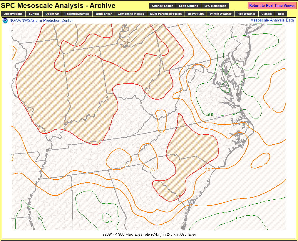
Mid-level lapse rates are important in judging instability when combined with boundary layer moisture content in the lower levels. With boundary layer moisture being poor for much of the MAF CWA today, the low to mid level temperature profile may be even more important, as it will define both convective inhibition and CAPE potential with a greater potential for inhibition with such a dry moisture profile. The convective forecast in MAF for the day featured generally weak forcing mechanisms, focused on orographic lift and a moisture gradient on the eastern side of the CWA. With any sort of convective inhibition, it would be difficult to forecast convective initiation away from the strongest forcing points until later in the day when convection is forecast to move in from outside the CWA.

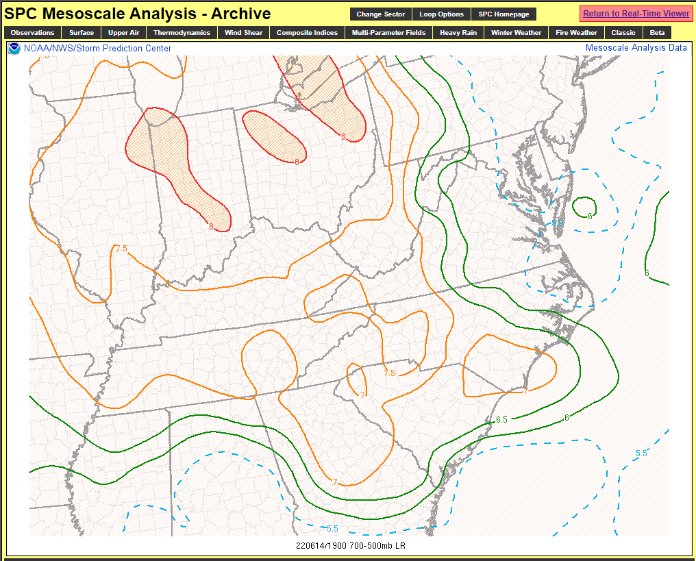
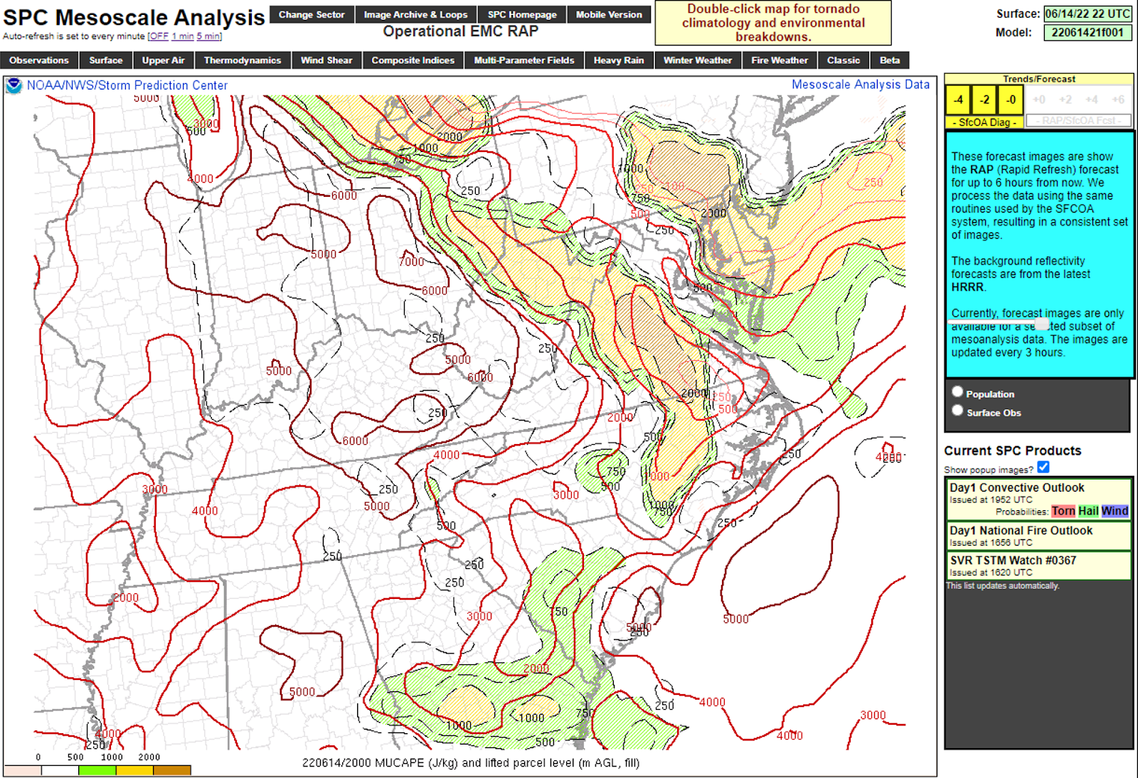
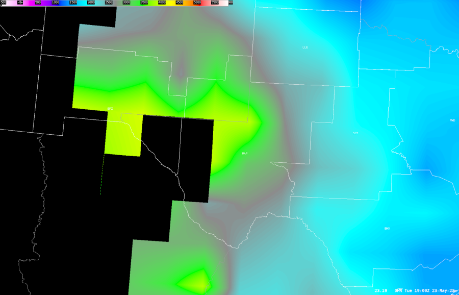
Shown below is the SPC mesoanalysis page depicting this afternoon’s 700-500mb lapse rates. The RAP guidance driving this page is showing very steep mid-level lapse rates of 8 to near 9.5 degrees/km over the MAF CWA. While steep mid-level lapse rates (indicative of cooler temperatures atop a warmer lower level air mass) are important for instability, very steep mid-level lapse rates could be due to a very warm low level air mass potentially creating a convective “cap” which may inhibit convection. With the very low surface dew points (into the 30s in some spots), a mid-level lapse rate exceeding 8.5 should mean convection struggles to initiate outside of areas of strong forcing.

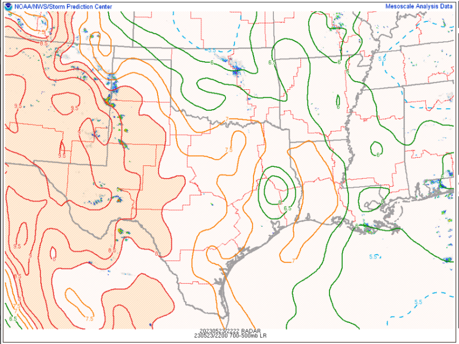
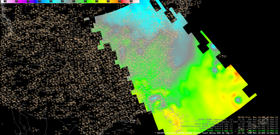
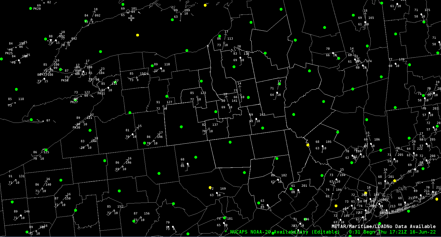
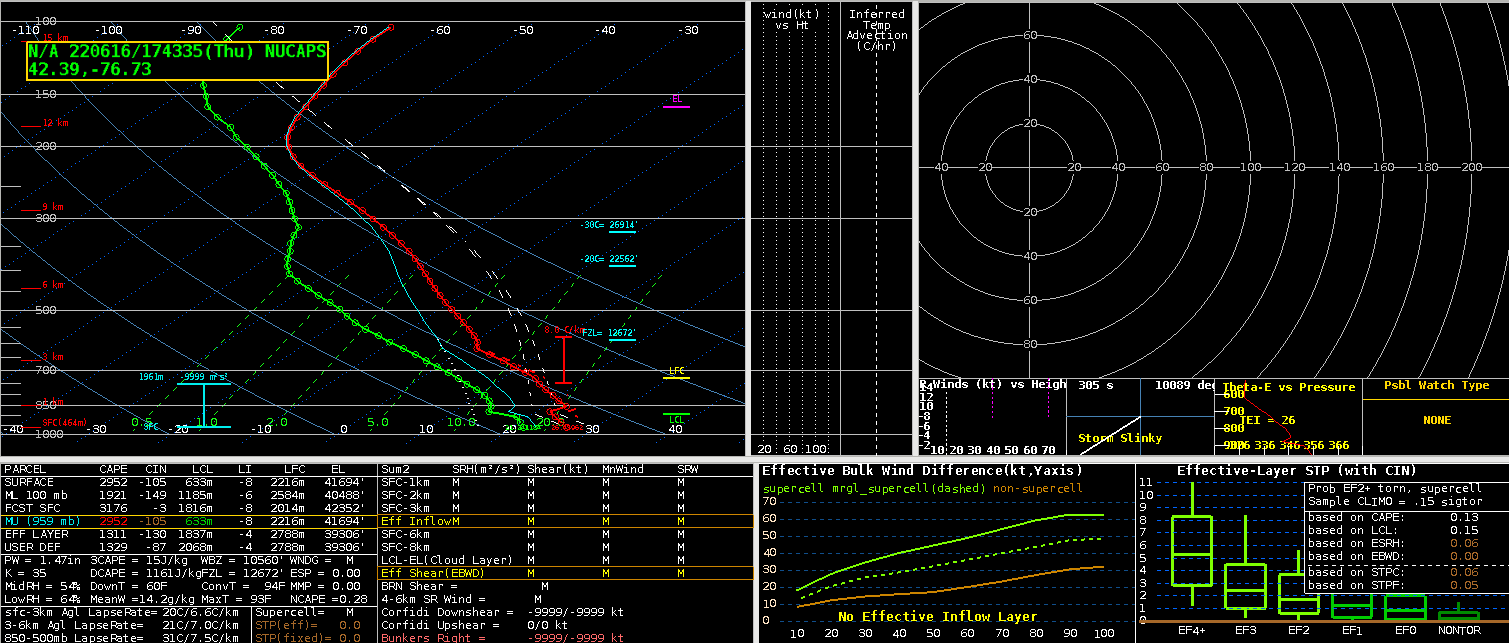
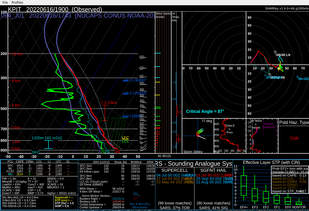
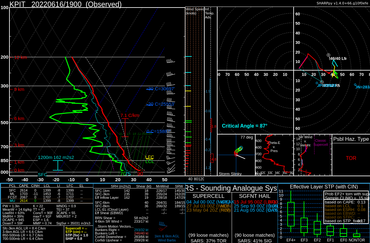
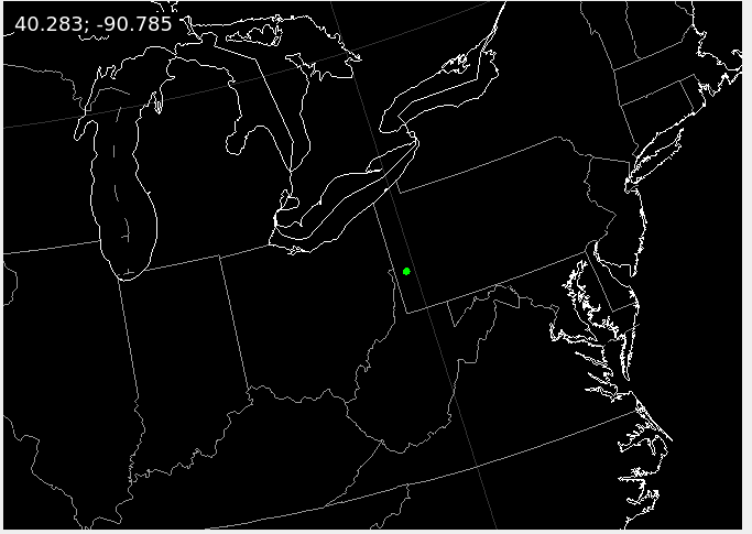
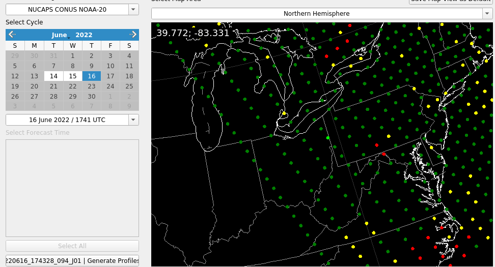
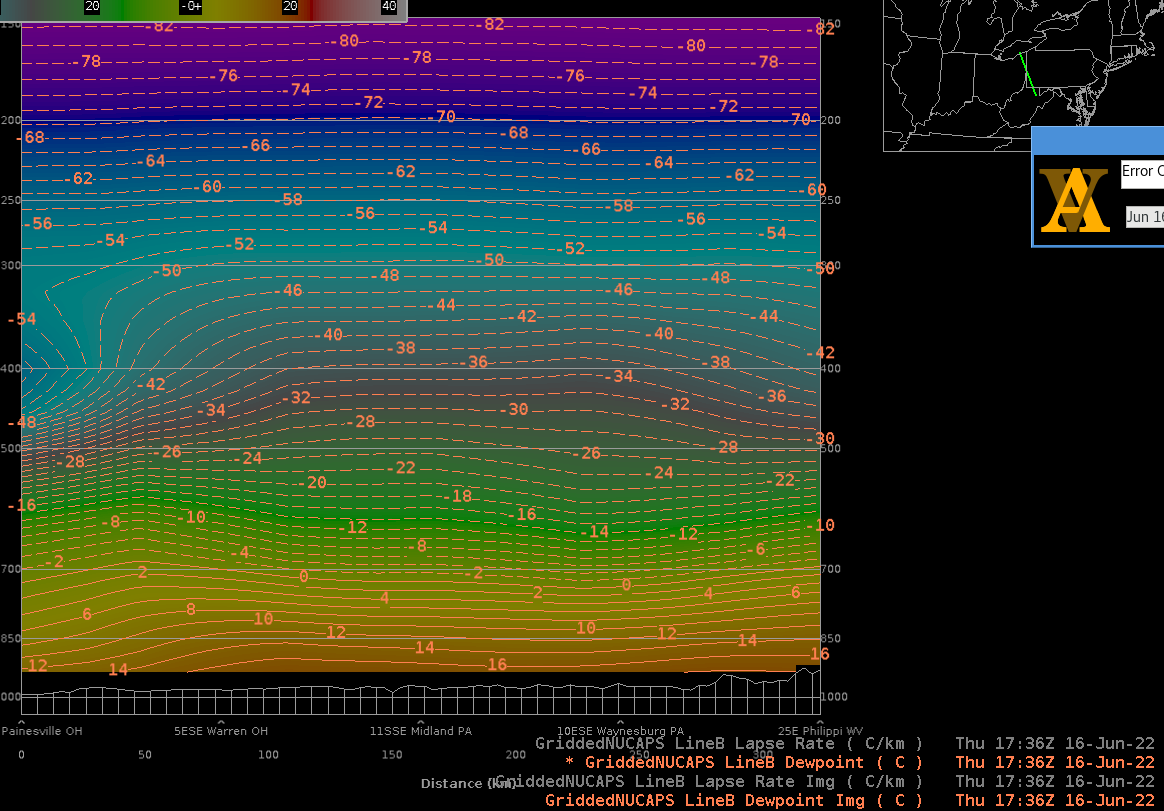
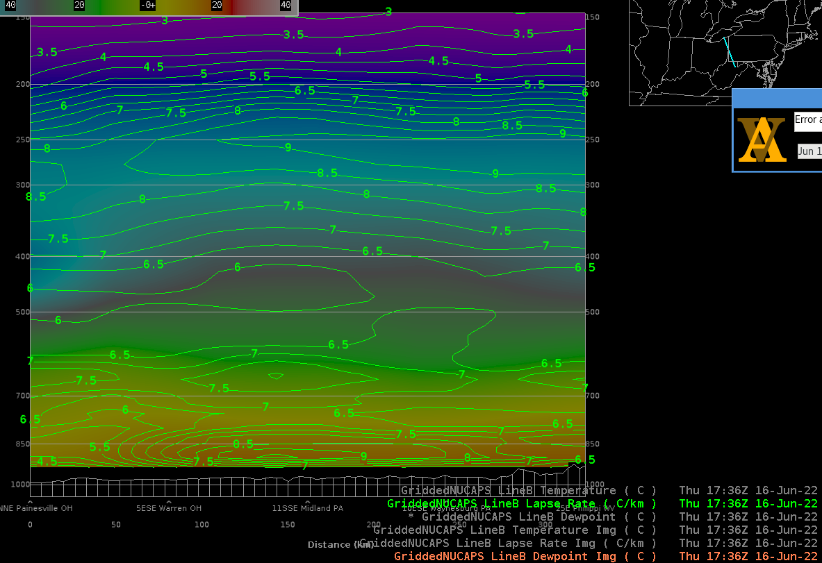
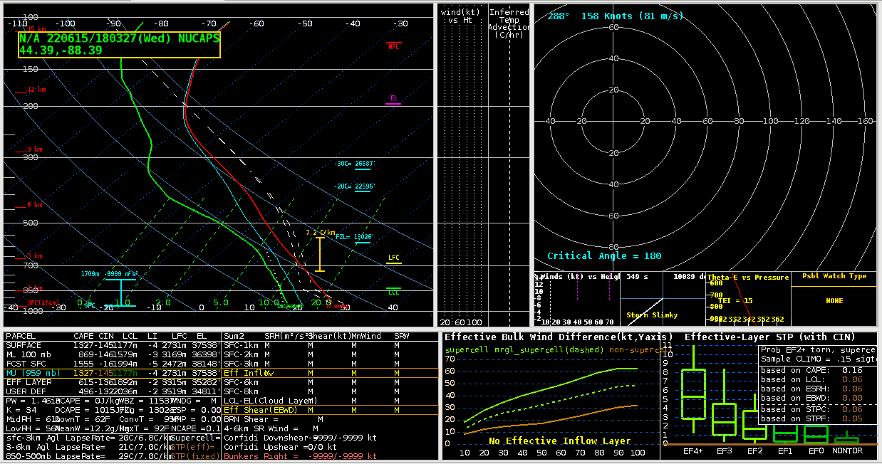
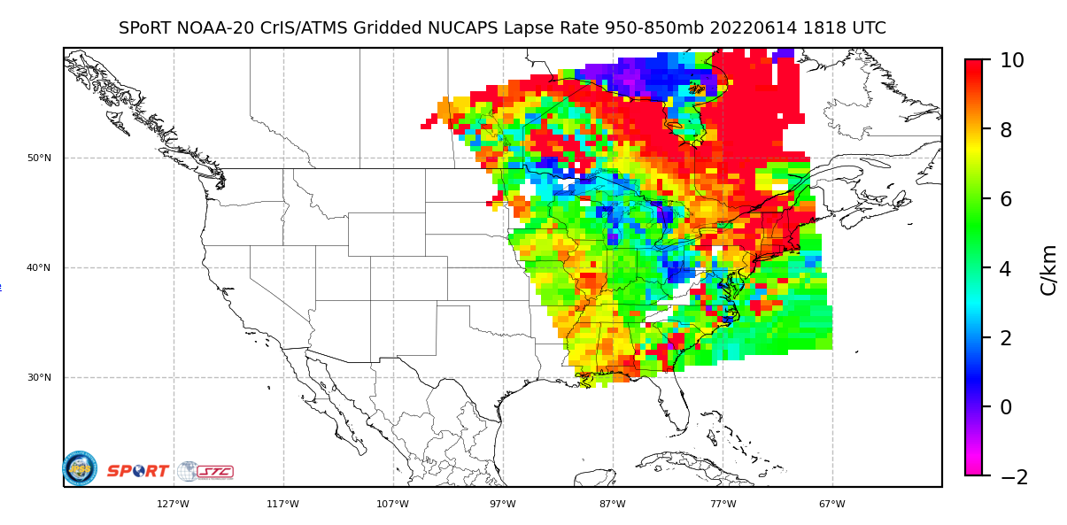
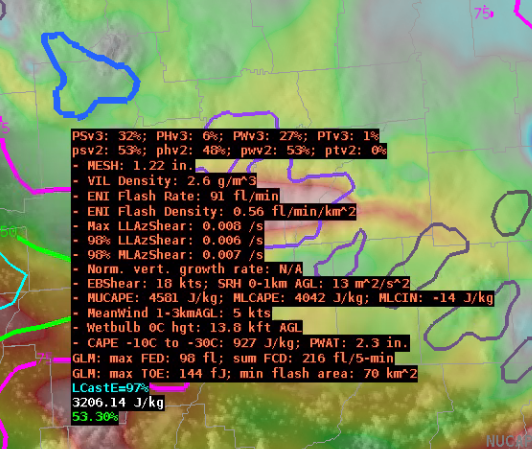
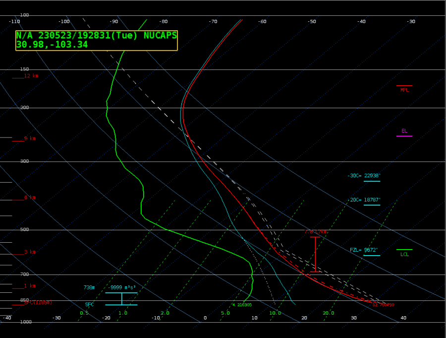
Looking at the afternoon NUCAPS satellite pass, it shows a fairly different picture for mid-level lapse rates over the MAF CWA. The observed lapse rates of 7 to near 8 degrees here are more normal for a convectively active environment compared to the 8.5 to near 9.5 degrees given by the RAP guidance.  It’s worth looking into how NUCAPS and guidance is handling temperatures at different levels to understand the differences between the lapse rates.

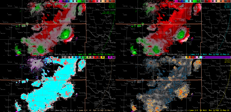
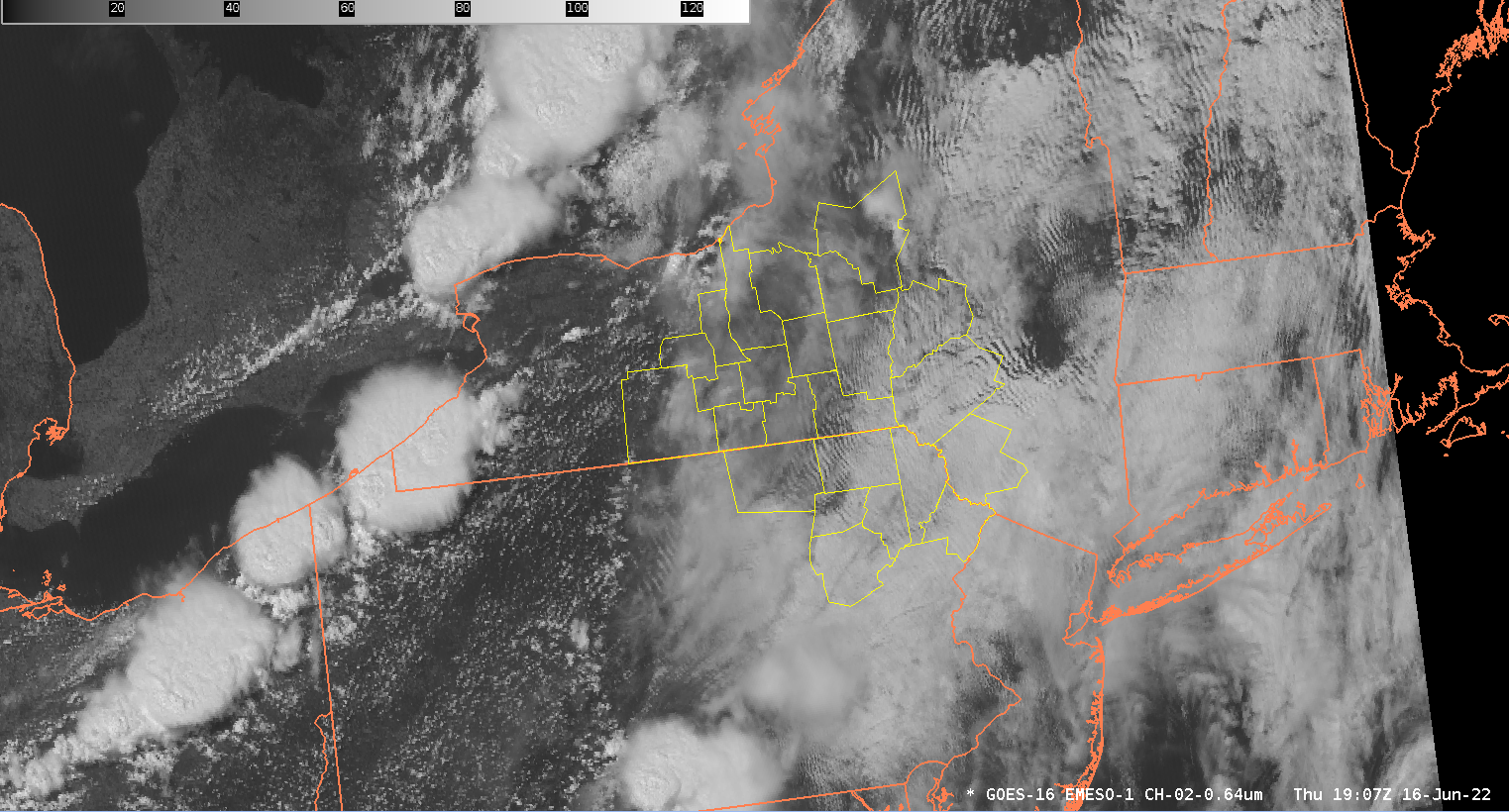
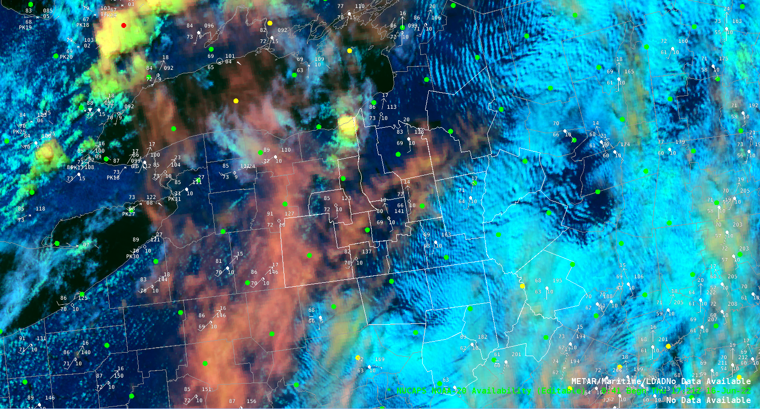
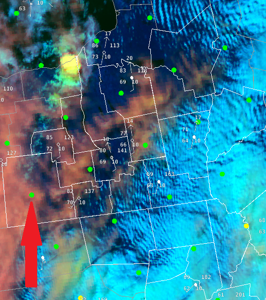
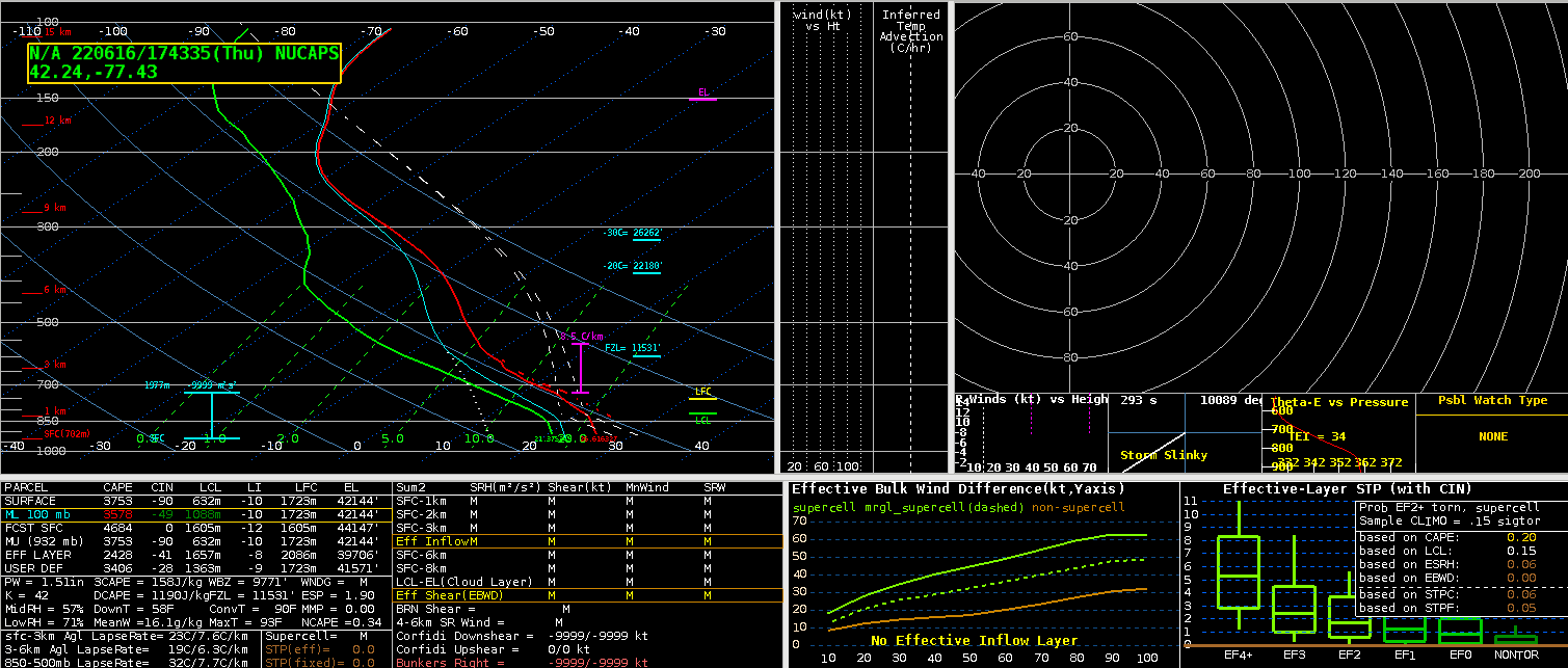
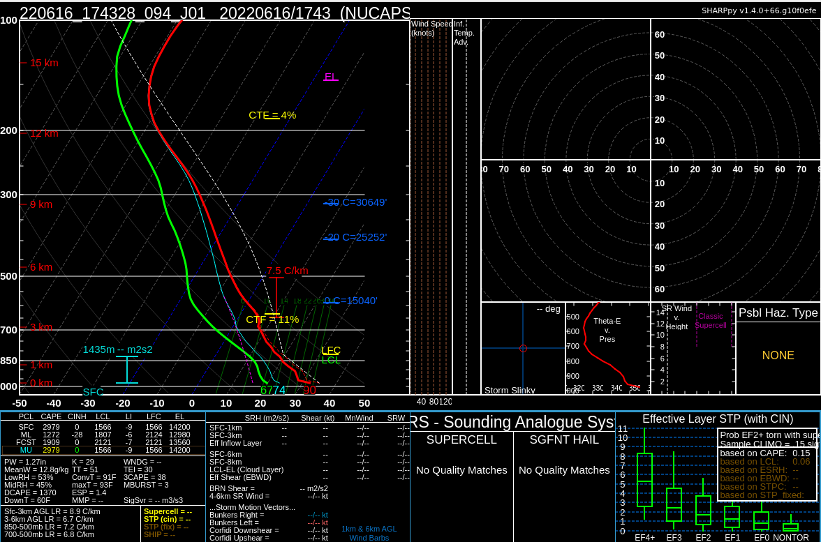
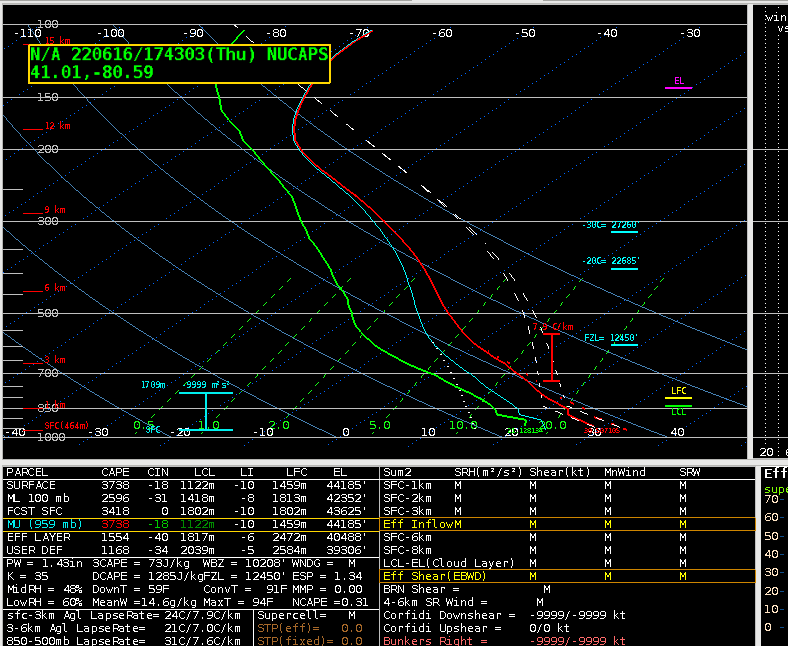
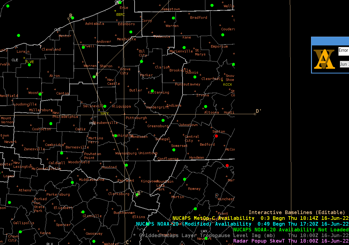
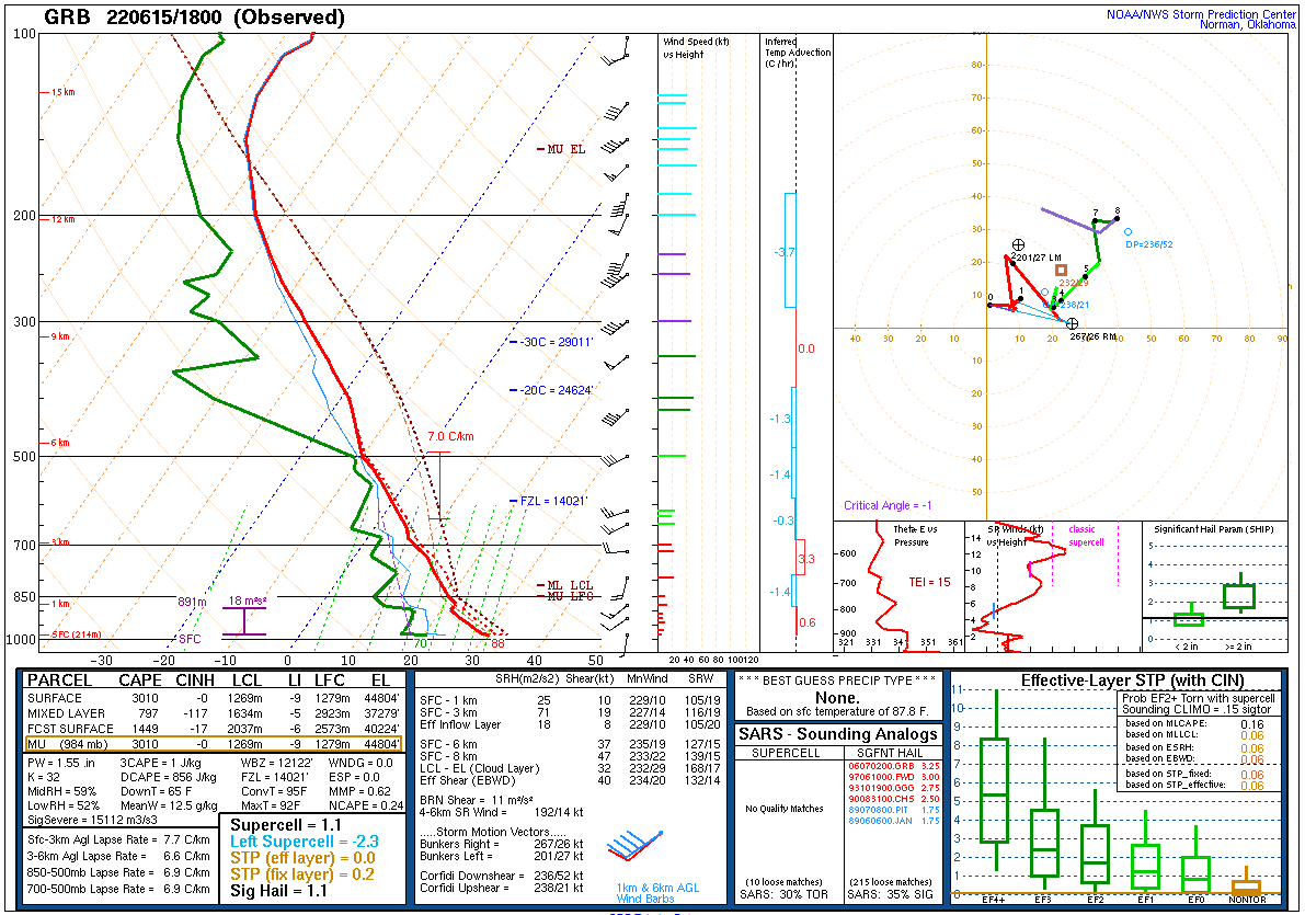
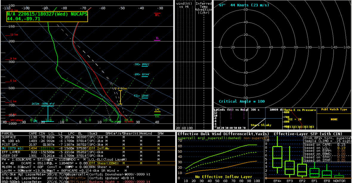
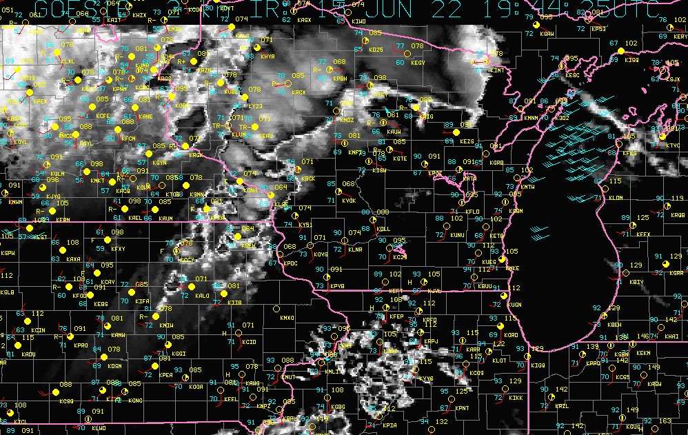
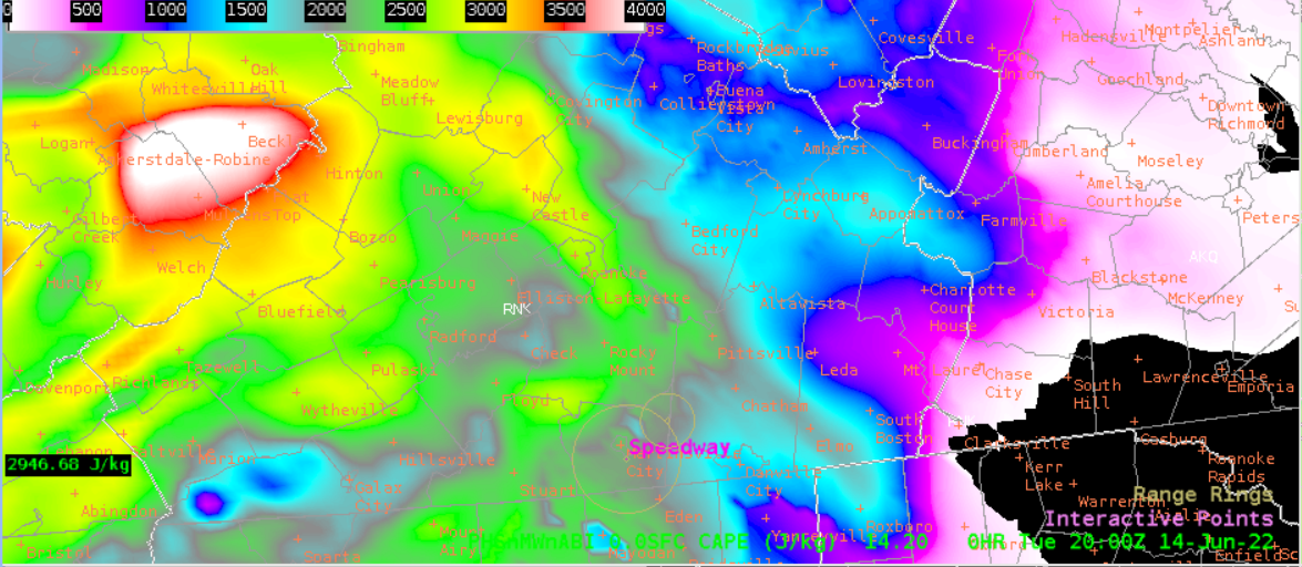
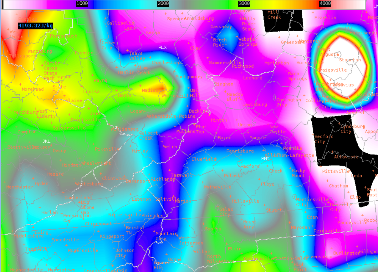
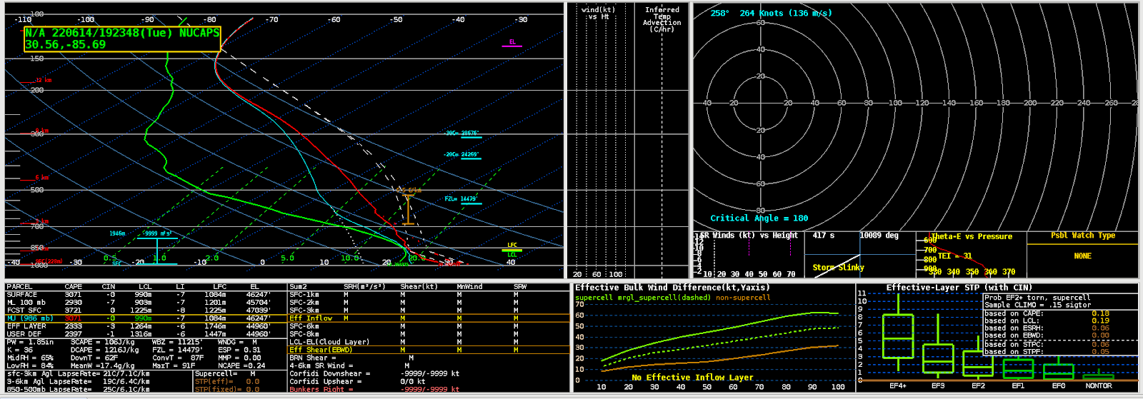
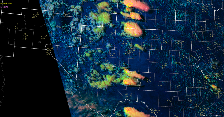
Shown below are both the NUCAPS sounding (first) and then the RAP sounding for a similar spot near the center of the MAF CWA. It’s interesting to note that it isn’t actually the 700mb temperature that is the main difference between the two soundings, but the 500mb temperature, with a 2-3 degree difference at 500mb. This could explain why there is still convection away from the previously discussed initiation points (such as out in the Fort Stockton area), however the warmer than forecast 500mb temperatures could be indicative of an environment that isn’t quite as unstable as forecast, and why the central MAF convection is notably weaker than convection well to the north in the Lubbock CWA. There are other contributing factors of course (weak surface convergence, very dry low to mid levels), but this is a major factor in judging updraft strength potential, and today lines up with where updrafts have develop but struggled to truly develop into strong or severe thunderstorms. The late afternoon Day Cloud Phase Satellite product shown below includes the non-severe convection in the south-central portions of the MAF CWA with the severe convection to the north (and their noticeably better defined anvil clouds).

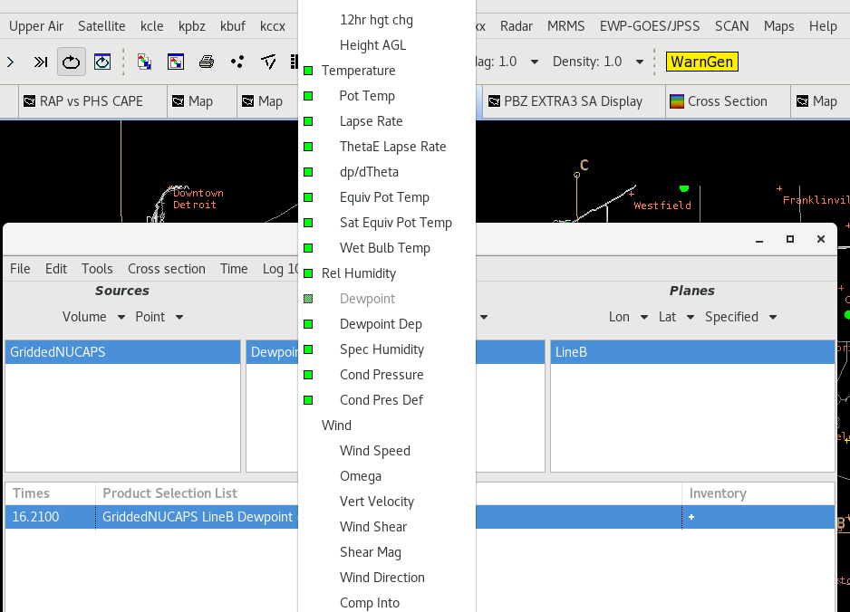
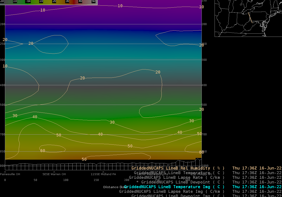
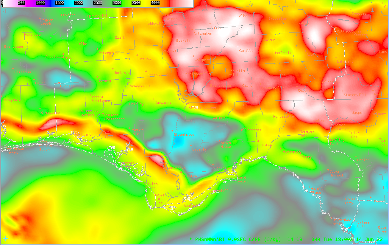
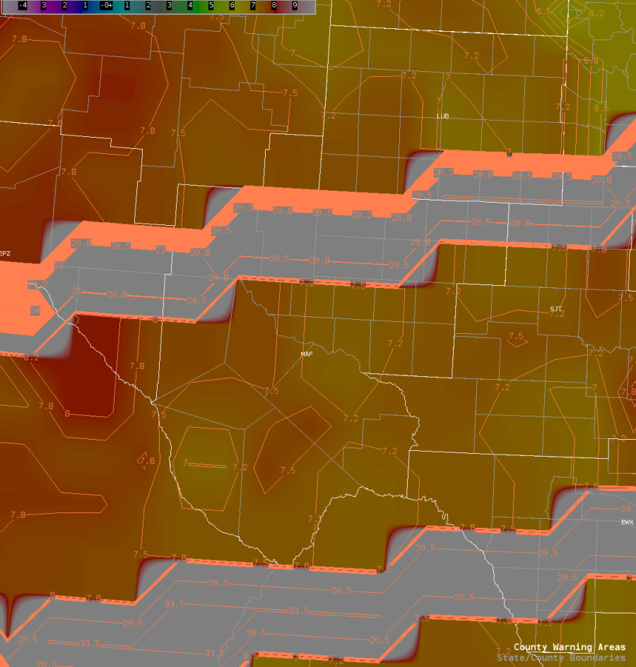
One quick screenshot to show is the NUCAPS LCL product, highlighting the better moisture on the eastern and northeastern edge of the CWA, lining up with the higher SPC risk.

-Joaq

Tags: None

Satellite HWT Day 1 Analysis Carl

PHS Model Analysis

PHS model struggled to properly capture convective initiation within the Texas Panhandle on the day. While it did see a few cells possibly starting, overall coverage was significantly underdone with many of these storms reaching severe thresholds including numerous reports of hail over 1″. The overall output shared many of the same struggles as the HRRR model on the day. Unclear what the exact problem was, but dry line convergence may have been better than in models on this day.

Above: 15Z PHS model output forecast for 17Z to 22Z from 5/22 with MRMS Reflectivity overlaid.

Below: 15Z PHS model output for 17Z to 22Z from 5/22.

NUCAPS Forecast

As I was beginning to test out these products, this caught my eye as a forecaster on the east coast that regularly deals with Cold Air Damming along the Appalachians. Models regularly struggle with multiple aspects of the dam, including extent, depth, and actual temperature and strength. Additionally, one of the most common pathways for large winter storms in the southeast is when low pressure passes across the Gulf Coast and into the Atlantic while an Arctic high in the northeast helps drive cold air damming into the area. Models again struggle with the dam, but also with strength of the warm nose aloft. I would love to see how this system performs in these scenarios – I know it isn’t “convective”, but it still is an incredibly impactful event, where the strength of the warm nose can be the difference between a few inches of snow or half an inch or more of ice. We regularly attempt to send up special soundings to get the best sample we can, but since GSP does not do a sounding, we rarely get a meaningful sample of the cold air damming in the SE states.

Above: NUCAPS Forecast from morning pass over east coast showing CAD feature over the east coast.

Octane Speed and Direction

Above: Octane image around 22Z for storm just south of AMA.

The Octane product was extremely useful in seeing when updrafts were really “taking off” and hitting the tropopause, immediately highlighting storms which require quick attention. Another extremely useful feature is sampling the actual speed, which gave a potential proxy for storm top divergence. Noticed that the Octane product gave a value around half of what the radar was measuring on this storm – ~50 kts on the Octane product vs ~100-110 kts on the radar. I’m assuming the resolution combined with some of the smoothing within the algorithm may be playing a role here, but it would be interesting to see if there is a consistent way to match the two up, even if there is just a “rule of thumb” or something. This would be huge in areas of sparse radar coverage (portions of the west or the ocean, for example).

Below: Radar image of storm top divergence near 22Z from KAMA.

ProbSevere v3

Noticed an interesting time period where two close updrafts – one fading, one picking up, resulted in some jumping of the ProbSevere product as it would sometimes combine the objects and then sometimes track them separately. I think this shows the importance of pairing the algorithm with analysis – just looking at the time series of the product could lead to misinterpretation of what was happening.

-Carl Coriolis

Tags: None

What’s the best way to look at NUCAPS?

So far this week, I’ve been impressed with the performance of NUCAPS and for the most part Modified NUCAPS with providing thermodynamic profile information in areas that there are overpasses.  However, what would be the best setup to figure out how well NUCAPS is doing.  Let’s dive in:

Today we’re located in Binghamton, NY (BGM) office with a Enhanced risk over the region.  We’ve also got a NUCAPS sounding directly over the region which can help us with evaluating how well things like the SPC Mesoanalysis graphics or other models are doing:

But, visible satellite shows that there are some clouds that could be interfering with the retrievals:

After playing around a bit, it may be a good idea to load the Day Cloud Phase RGB, NUCAPS points, and surface observations into one pane:

This is useful for three reasons:


  1. We can see that the red in the Day Cloud Phase are mainly high clouds that are pretty thin and has enough gaps to allow for good retrievals underneath the cirrus.
  2. The low clouds are pretty thin except over the southern part of the CWA where some of the retrievals are yellow indicating that caution should be taken when looking at the profiles
  3. The surface observations can be used to give an idea of how well the surface T/Td are in the soundings which will impact all of the convective parameter calculations (especially CAPE/CIN)


So what about the soundings?  Looking at the NUCAPS and Modified NUCAPS here:

We can see how things are handled by the soundings.

Here is the original NUCAPS sounding at this point:

Of note, the surface conditions in the NUCAPS sounding is too warm (85 vs 80 at the nearest ob) while the Td were fairly close 69 vs 70.  How did the modified NUCAPS do?

80/70 in the sounding which is a much more likely scenario based on surface observations closest to the time of the overpass/sounding.

Why is this important?  Well, all your convective parameters are based on these two conditions.  MLCAPE drops by around 400 J/kg (~3900 J/kg vs ~3500 J/kg) AND CIN increases from -19 J/kg in the unmodified to -49 J/kg in the modified NUCAPS.  This too lines up with what the visible satellite shows; a lack of boundary layer CU potentially meaning the CAP is holding strong.

-Pym

NUCAPS sounding comparison vs observed 19z PIT sounding.

With the threat for severe weather today, WFO Pittsburg launched a 19z special sounding to access the atmosphere. The atmosphere featured a moist boundary layer with dewpoints the lower 70s and decent lapse rates throughout much of the atmosphere of around 7 C/km. The low-level wind profile in the observed sounding indicates veering winds with height and low level winds generally from the west southwest to west. The wind profile was helpful in determining the severe weather threat. Based on this low-level wind profile, one can conclude that the tornado threat appears to be fairly low.

There was also a NUCAPS pass across the region around 1741 UTC. I selected a point just to the west of the Pittsburgh office based on the general atmosphere advection to the west based on the observed sounding. Due to this, it would seem that the point just to the west of Pittsburgh at 1741 UTC would be a good approximation of the atmosphere near the Pittsburgh area at the time of the 19 UTC sounding.

The Observed sounding indicates major fluctuations in the dewpoint temperature throughout the atmosphere but the NUCAPs sounding indicates a much smoother moisture profile. Overall, these different methods indicate rather similar PW values to the observed around 1.31 inches and NUCAPS PW of 1.27 inches. Overall, a fairly consistent moisture profile. There are some noticeable differences in the boundary layer moisture profile. The modified NUCAPS is included as the last image. It seems that the modified NUCAPS introduces a bit too much moisture with PW values of 1.43 inches. These higher PW values also lead to higher values of instability as well.

Overall, the NUCAPS sounding was helpful in diagnosing the thermodynamic profile of the atmosphere. It also arrived over an hour earlier than the observed sounding. The sounding indicates a moderately unstable atmosphere across the region capable of leading to severe weather. The moisture profile is smoother in the NUCAPs but it doesn’t seem to affect the overall moisture with PW values being the same. It would be nice to add a model wind profile to the NUCAPs sounding. This way it would be possible to access the tornado threat as well because there is not much available in the thermodynamic profile alone to make this assessment. However, I’m very impressed by the similarity between the NUCAPs and observed sounding.

Observed 19 UTC PIT sounding and NUCAPS from 1741 UTC.

19 UTC PIT Observed Sounding

Location of Observed 19z PIT sounding.

1741 UTC NUCAPS Sounding.

1741 UTC NUCAPS soundings point, brighter green dot.

1741 UTC Modified NUCAPS.

– Marty McFly

Gridded NUCAPS Cross Sections

It took until the end of the week to think of trying this, but it turns out that the AWIPS cross section tool works with gridded NUCAPS (and it turns out some folks have already been using it). Mainly this suggests the usefulness of gridded NUCAPS at spatially comparing many sounding points (rather than the somewhat klunkly process of loading many soundings into NSHARP).

Here’s the cross section used to sample the ~1730Z NOAA20 NUCAPS soundings (lineB). Initially I thought the cross section would actually interpolate the 7 sounding points, but later I realized that the griddedNUCAPS would be sampled across the lineB.

The AWIPS volume browser (in cross section mode) allowed me to select griddednucaps as the source, and then both native and several derived parameters for display, and then of course the baseline (i.e. lineB) along which to calculate the cross section.

The main challenge with this workflow is knowing to find the exact time where your griddedNUCAPS is valid.  I loaded up griddedNUCAPS in a regular D2D panel to see that it was valid at 1730Z, then I increased the framecount of my cross section enough to allow me to step back in time to that point. Then, voila… I was able to plot images and/or contours across the line I’d drawn on the map.

Above: Cross-section of griddednucaps over ~7 sounding points, showing dewpoint as both image and contour

Above: Cross-section of griddednucaps over ~7 sounding points, showing dewpoint as image and lapse-rate as contour

Above: Cross-section of griddednucaps over ~7 sounding points, showing Temperature as image and relative humidity as contour

– Buzz Lightyear

Pre-Convective Environment Across GRB

With a busy day still underway across Wisconsin, the use of the Optical Flow Winds, GLM, Prob Severe, and NUCAPS soundings were a big help in looking at the pre-convective storm environment and in warning operations.

When it came to looking at sounding data we had a NOAA-20, and AQUA pass for the polar orbiting satellites, that we could then compare to the special observed sounding from GRB.

There are some spatial differences in the locations since each satellite doesn’t pass over the exact location and the observed sounding came from the GRB office. I ended up grabbing NUCAPS soundings from west of the office where I thought the better storm environment would be. Regardless of this they do show great information over a temporal and spatial scale.
Just between Aqua (bottom image) and NOAA-20 (middle image) you can see that the environment becomes much more moist over time (AQUA came around 19Z and NOAA-20 came around 18Z). The increase in temperatures and dew points in the low levels between the two NUCAPS soundings show that there was increasing low level lapse rates and increasing CAPE through time. Then compare both of these to the special sounding sent out by GRB, you can see AQUAs vast improvement in the low level over NOAA-20. The one caveat seems to be the smoothing of the values in the mid levels. Smoothing seems to have decreased the values almost too much for both satellite soundings. It is fairly within reason given that there is a dry layer in the mid levels on the observed, but the smoothing looks to have slightly overdone it.
Moving on to the GLM, it was very helpful when boosting confidence in the warning operations. There were lightning spikes collocated with increasing rotation and reflectivity. The one things worth mentioning is to have a reminder or maybe even have offices lower/change the color curves for FED prior to the start of an event. It could even be a permanent change that some offices make.
Since I was the only one in the group to check, compare, and lower the FED color curve accordingly it was much easier to pick out lightning jumps. From the graphic above alone, 0-65 was much more informative than 0-128 or 0-260.
The last thing worth mentioning for the day was the Optical Flow Winds. While this was helpful in a warning environment to look at storm top divergence and speed of the winds at the tops of clouds, I was able to find another great use for it. In the pre convective environment I had pulled up the Optical Flow Winds and noticed that it was tracking winds and speeds of clouds over Lake Michigan. In an area where any wind information and observation data can be very sparse to near non-existent. The optical flow winds could be very helpful for open waters forecasting.
-Cirrus Fields

NUCAPS Sounding Verification – Day 3 (June 15, 2022)

I had a great opportunity to get some verification on a NUCAP sounding that passed through shortly after 19z on June 15, 2022.  It was the NOAA-20 which just happened to pass over eastern Iowa where the DVN WFO launched a special sounding at 19z on the same day.  I’d estimate the locations of the two soundings compared were roughly 50-60 miles apart. The DVN sounding was equidistant from 4 NUCAP soundings and all those soundings had very similar readouts from one another (see Figure 1).  One of the disadvantages of the NUCAP soundings is no winds are measured, but there are plenty of other parameters that could be compared from the two soundings. The first thing that I compared were the CAPE values (See Table 1).  The other two tables below compare other various parameters.

Some interesting differences between the CAPE values measured. Uncertain why the NUCAP sounding doesn’t suggest any 0-3CAPE values, especially since the much larger surface based CAPE.  Another big difference that really stood out was the freezing level heights and the Convective Temperature. Obviously the NUCAP sounding may have overestimated the temperature profile and thus larger CAPE values, but I found it interesting that the freezing level from the NUCAPs sounding was slightly lower. The RH values were fairly similar, particularly the midRH values, but also eyeballing the dew point temperature profile, they are pretty close near the surface.

Overall, I do like the NUCAP soundings availability as it is another tool available for the forecast toolbox.  It might be wise (as with all things meteorology) to be careful with totally believing some of the NUCAP sounding readings after seeing this comparison.

Table 1: CAPE parameters compared from 19z soundings.  (J/kg)


Table 2: Comparing various parameters found in soundings. Note: LCL, LFC, LI, etc are all measured from the surface.


Table 3: Comparing various lapse rates and -20C/-30C heights.


Figure 1: Location of the DVN 19z special sounding and the NUCAPS NOAA-20 1921z sounding.

Figure 2: DVN special sounding launched at 19z on Jun 15, 2022.

Figure 3: NUCAP NOAA-20 sounding at 1943z on Jun 15, 2022.

– PODIUM

The utility of satellite derived data in mesoanalysis & near term convective forecasting

The most common mesoanalysis tool is the SPC (RAP) Mesoanalysis Page

While there was no new convection in the operational period for the RNK CWA, satellite based products did show their utility as a cross check with the SPC Mesoanalysis. Since the SPC Meso-a page starts with a RAP model background field, the ability to QC check this data will be helpful in gauging the accuracy of hourly RAP and HRRR model fields. In this way, you can gauge whether the Mesoanalysis and hourly updating fields are either on track or likely vary in meaningful ways from satellite derived data.   Having this data will be especially useful in locations that do not have frequent or any aircraft vapor soundings.

Mid-level lapse rates

SPC Meso-A 700-500 mb lapse rates at 19z 6/14

NUCAPS 700-500 mb lapse rates at 1819z 6/14

Excluding the likely unreliable data in the region of lingering cloud cover across central Virginia, the NUCAPS data roughly ranged from 6.5C to 7.6C/km across the RNK CWA, which is fairly close to the SPC Meso-A 700-500 mb lapse rates. Within the past few years, maximum 2-6 km AGL lapse rates were added to the SPC Meso-A page. The question I had was, with its good mid-level moisture sampling, would a NUCAPS sounding be a good QC check for the SPC max 2-6 km AGL LR field? Examples are shown below.

SPC Meso-A Max lapse rate (C/km) in 2-6 km AGL layer at 19z 6/14

NUCAPS sounding near Martinsville, VA at 1819z 6/14

As you can see from the SPC mesoanalysis graphic, there was a region of 7.5 C/km to 8.4 C/km maximum lapse rates in the 2-6 km AGL layer. The NUCAPS sounding above sampled a layer of 7.9 C/km lapse rates from just below 700 mb to just below 500 mb, which verifies the SPC Meso-A field.

CAPE analysis

SPC Meso-A SBCAPE and SBCIN at 20z 6/14

SPC Meso-A MLCAPE and MLCIN at 20z 6/14

SPC Meso-A MUCAPE and LPL at 20z 6/14

Here we’ll compare the SPC Meso-A graphics to the PHS initialization at the same hour.

PHS SFC CAPE at 20z 6/14

In general, the CAPE values on the satellite derived initialization is less aggressive the SPC Meso-A SBCAPE, but the distribution is similar, showing a west to east gradient, with lower values east where there remained lingering debris cloud cover. The MLCAPE and MUCAPE fields show a similar west-east gradient in CAPE, while SBCIN and MLCIN are also maximized in the cloud cover area across central VA.

The gridded NUCAPS MAXCAPE field was from the 18z hour per 1819z sounding availability, and was noisier data as would be expected due to unreliable retrievals under thick cloud cover.

Gridded NUCAPS MAXCAPE at 18z 6/14

Excluding the bullseye to the northeast, the distribution on the NUCAPS compares favorably to the SPC Meso-A MUCAPE field. Furthermore, recalling the NUCAPS 1819z sounding near Martinsville, MUCAPE values over that area on the SPC Meso-A field vs. the NUCAPS sounding match up well. While the time difference between the NUCAPS and SPC Meso-A fields is something to take into consideration when using the data, the less than 2-hour difference between them helps in this case. Furthermore, if we were using the NUCAPS data to compare to the SPC Meso-A graphics, we would’ve done a direct 18z check as well.

– Hurricane84

Storm Movement and Severity at TAE

Down in Tallahassee, there are two boundary layers where storms are initiating or ongoing.  There is a lingering MCS that moved down from the Midwest overnight and a Sea Breeze. You can see the CAPE gradients along the both boundaries and how that progresses forward in time with both the boundaries interacting with one another.

17Z

18Z

19Z

This tracks very well when you overlay the visible satellite imagery with the PHS images as you can see the cumulus field along the CAPE gradient. This gives a good visualization of where storms are initiating along the Sea Breeze and the strongest storm movement along the MCS.
As these two boundaries move closer together they will be moving into a more favorable low level environment. It would be nice to have the Polar Orbiting Satellite NUCAPS sounding data available. This way we could verify lapse rates and what Prob Severe is giving us. While an upper level ridge is in place over the southern CONUS what sounding information we did have early on in the forecast period was very helpful as outside of the storm environment skies were clear. I was able to grab some gridded NUCAPS data that shows the diurnal destabilization of the low levels from 18Z. Now that it is 21Z, that data isn’t as helpful in either a warning or pre convective event because things could have changed drastically in the 3 hrs since the last Polar Orbiter moved through.
After overlaying Prob Severe with the PHS CAPE and Visible Satellite imagery, you can see your strongest storms along the CAPE gradient which tracks well. However, there are differences between Prob Severe Version 2 and Version 3.
A great example of the differences between PSv3 and PSv2 is with one of the strongest storms of the day for the Tallahassee CWA. Version 2 seems to try to highlight a hail threat at 48% while Version 3 has prob severe hail at 6%.  It seems that Version 2 is overestimating the Hail threat for this area. Especially given the subpar mid level lapse rates at 5 C/km or less, storm motion of around 5 kts or less and the upper level subsidence. The storm environment just is not conducive to produce quarter sized or larger hail.
– Cirrus Fields

NUCAPS Sounding Feedback – Day 2

One of the first things that I realized that became a challenge when experimenting with the NUCAPS soundings was when after you load up one from the map, Nsharp loads up in another tab automatically.  This is totally fine, but a nice feature would be to show the location of the dot that you clicked on. This might be in a small map located in Nsharp.

Another cool feature (in AWIPS) would be to maybe highlight the dot that is already loaded in Nsharp on the planview map.  Because when you go back to the planview to click another dot, I’d forget which one I already loaded.  I guess to help this, another option would be to have the capability to load up multiple dot soundings and toggle them off and on.

Lastly, a feature I’d love to see are winds in these NUCAP soundings.  Winds are an extremely powerful tool when forecasting severe storm mode, storm motion, etc.  but also it would be helpful to identify levels of turbulence and even LLWS.  If we could see areas where there might be moderate to severe turbulence, this is great information to air traffic controllers in order to divert aircraft to different levels or north/south of those strong winds.

Podium