Supercells and Optical Flow Winds

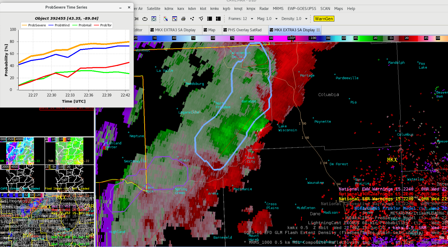
With the storms moving out of La Crosse’s CWA, I’ve got a bit of time to finally take a look at the Optical Flow Winds.  I’m intrigued by the product to say the least.

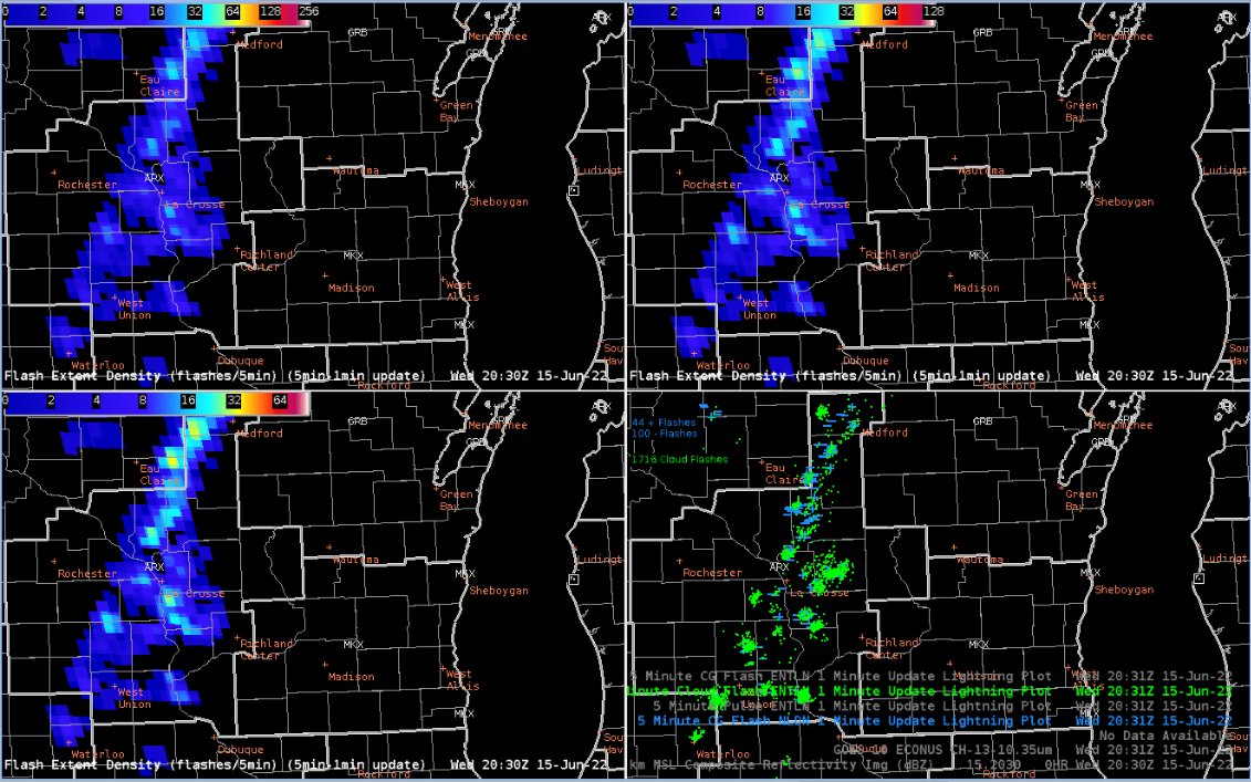
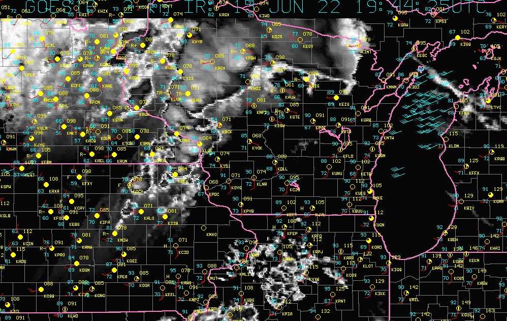
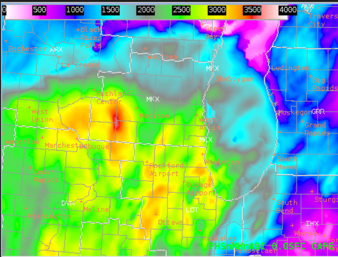
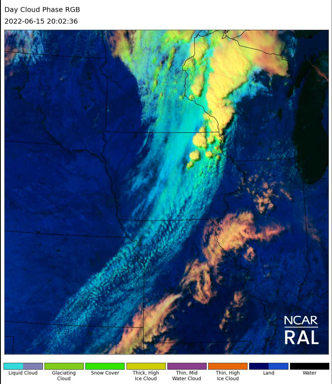
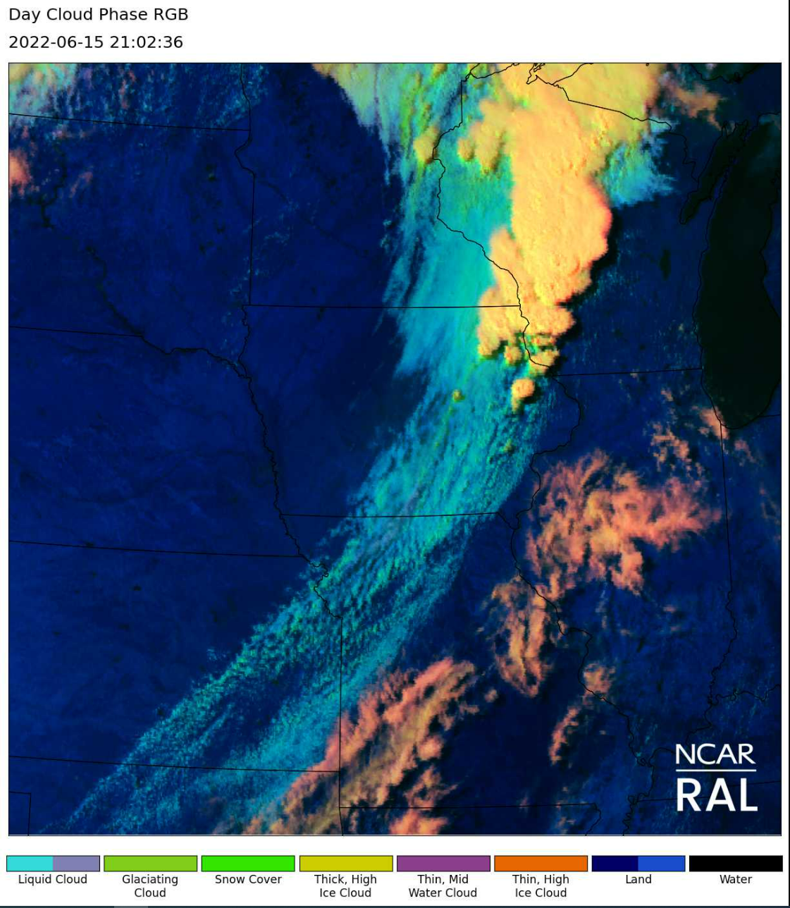
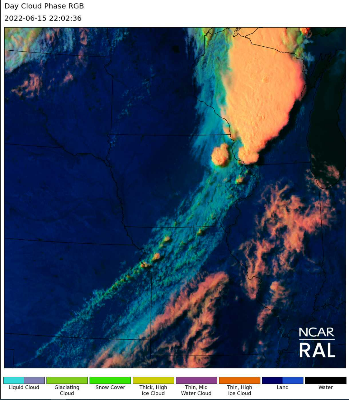
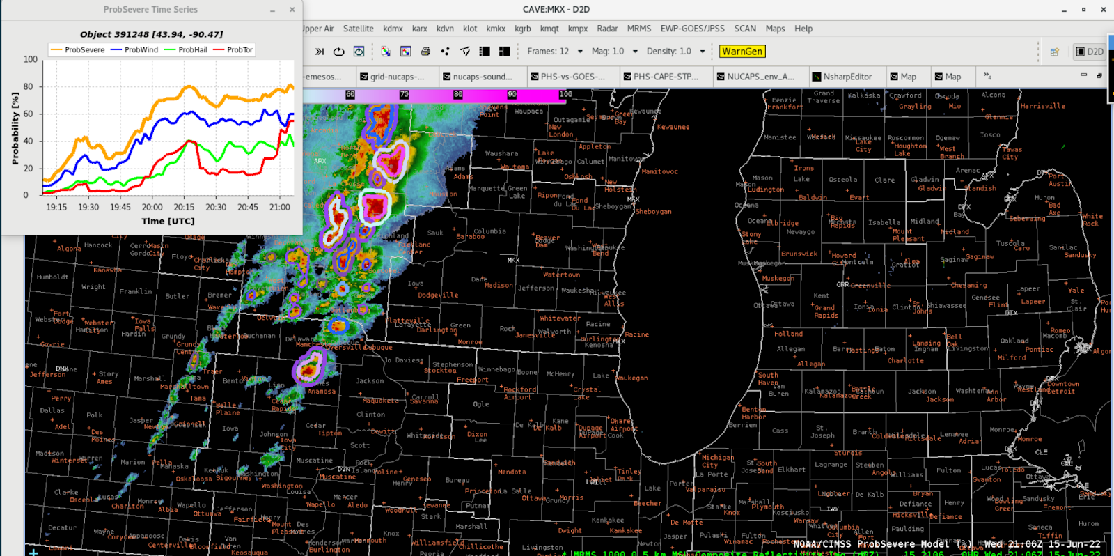
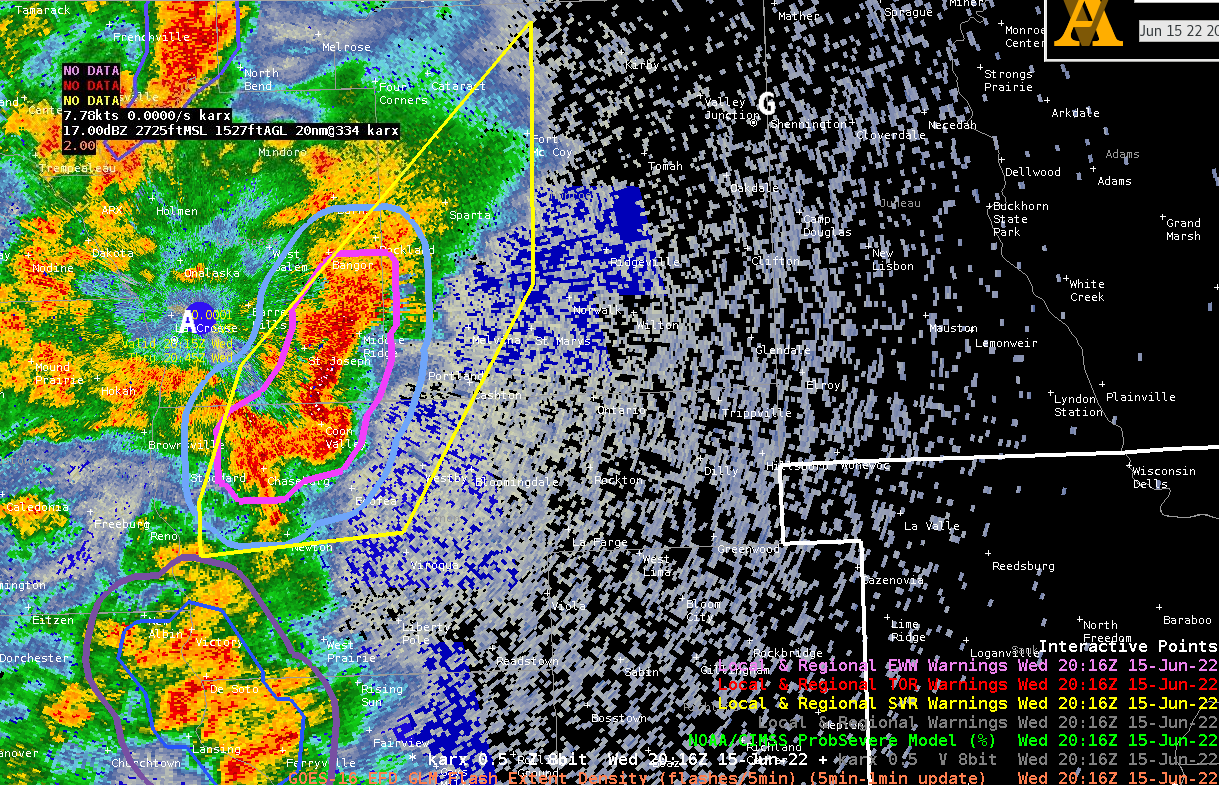
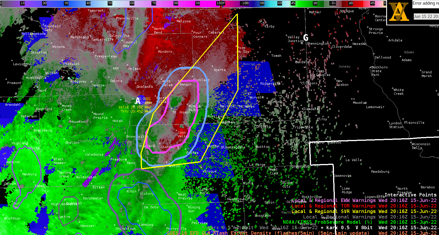
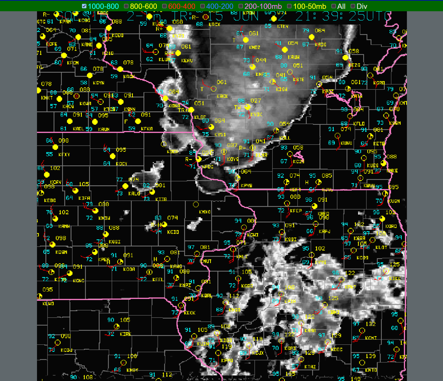
Here is a still image of the GOES-East Meso1 sector today with the string of supercells ongoing (and tail-end charlie in NE Iowa).  One thing I was curious about was how well this could detect storm top divergence.  The radar data was pretty noisy in AWIPS so it was hard to see this in those products.

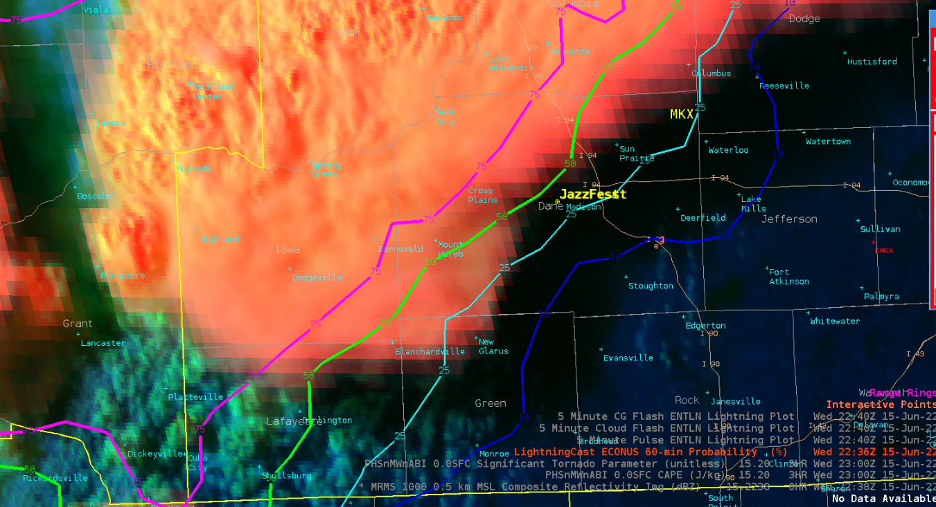
Here is what the “base” product shows.

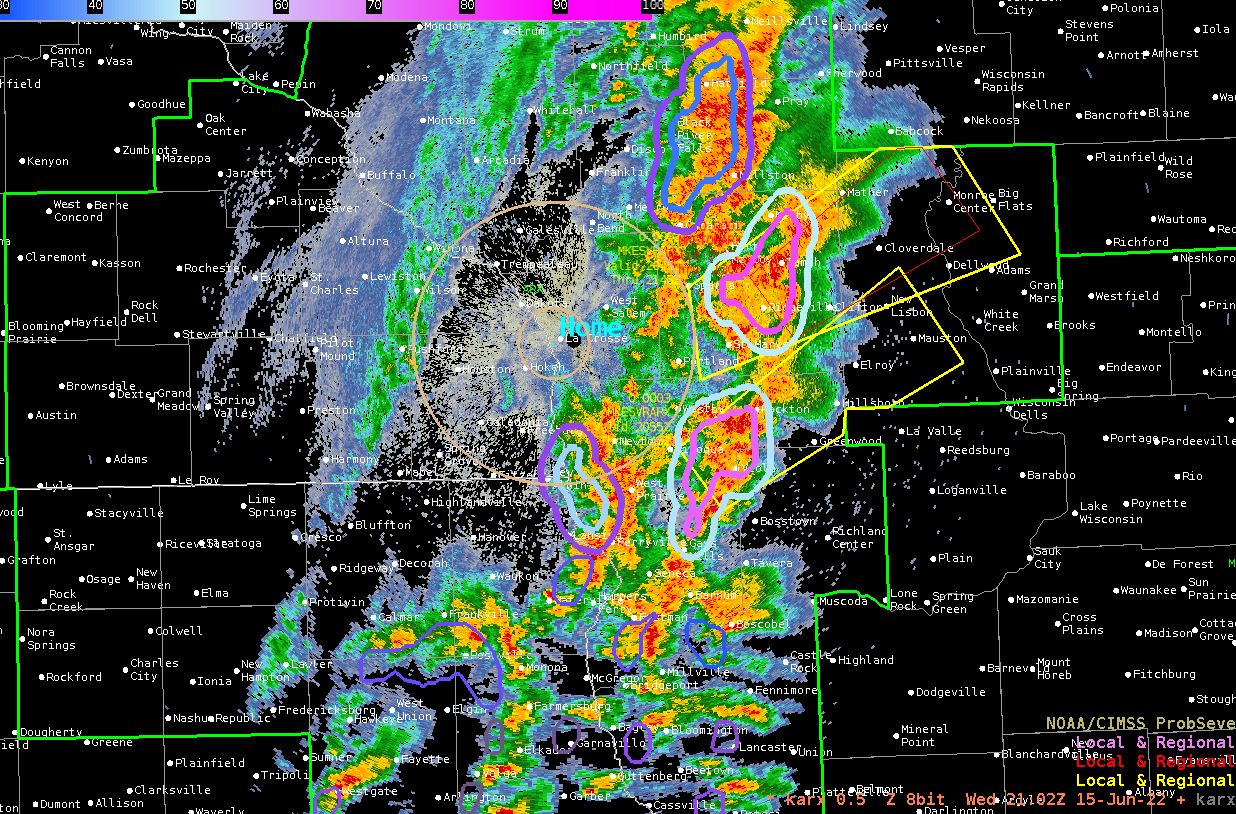
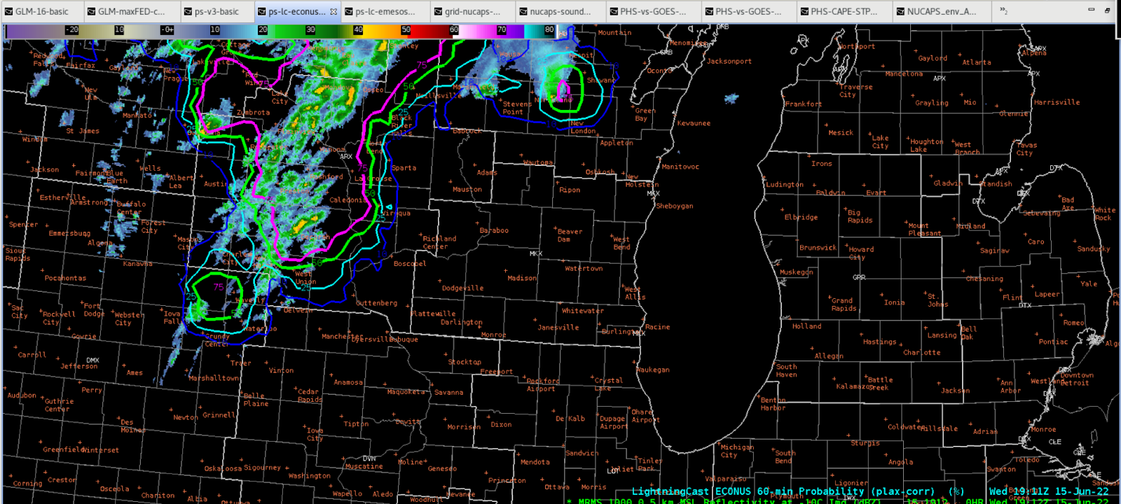
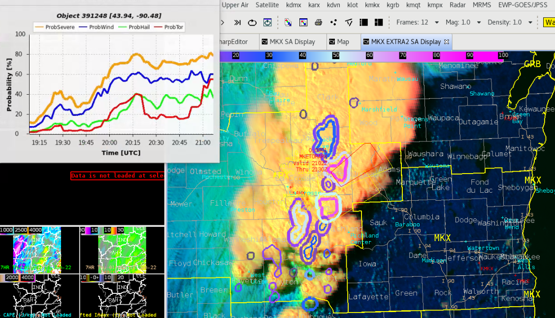
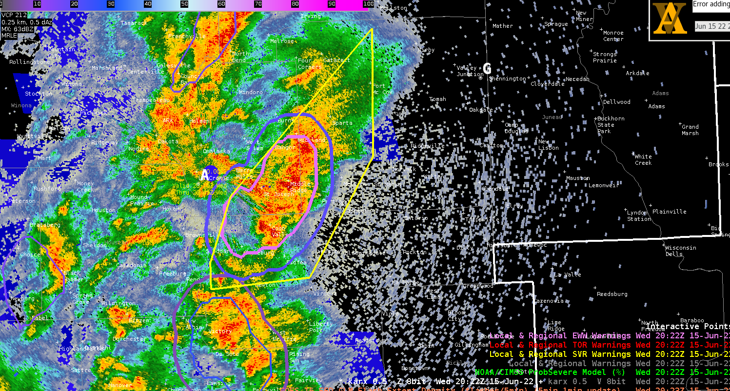
Now let’s overlay the upper-level winds as detected by this product (roughly the 100-50 hPa layer although I wouldn’t be surprised if some storm tops are going above this:

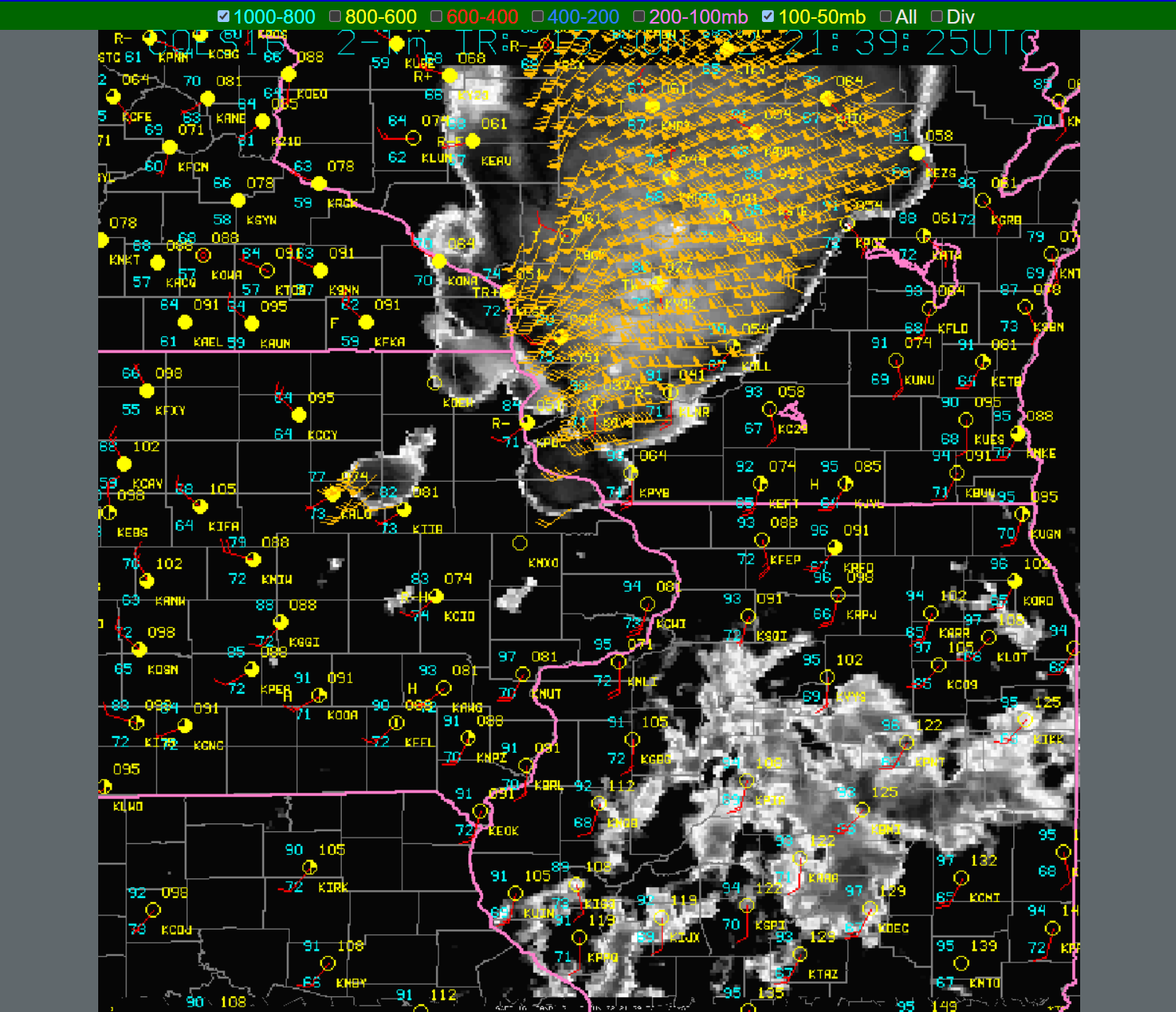
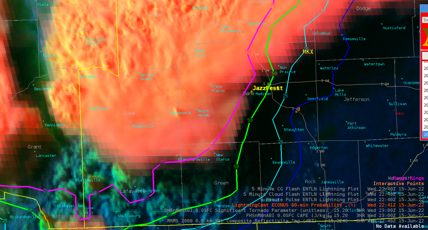
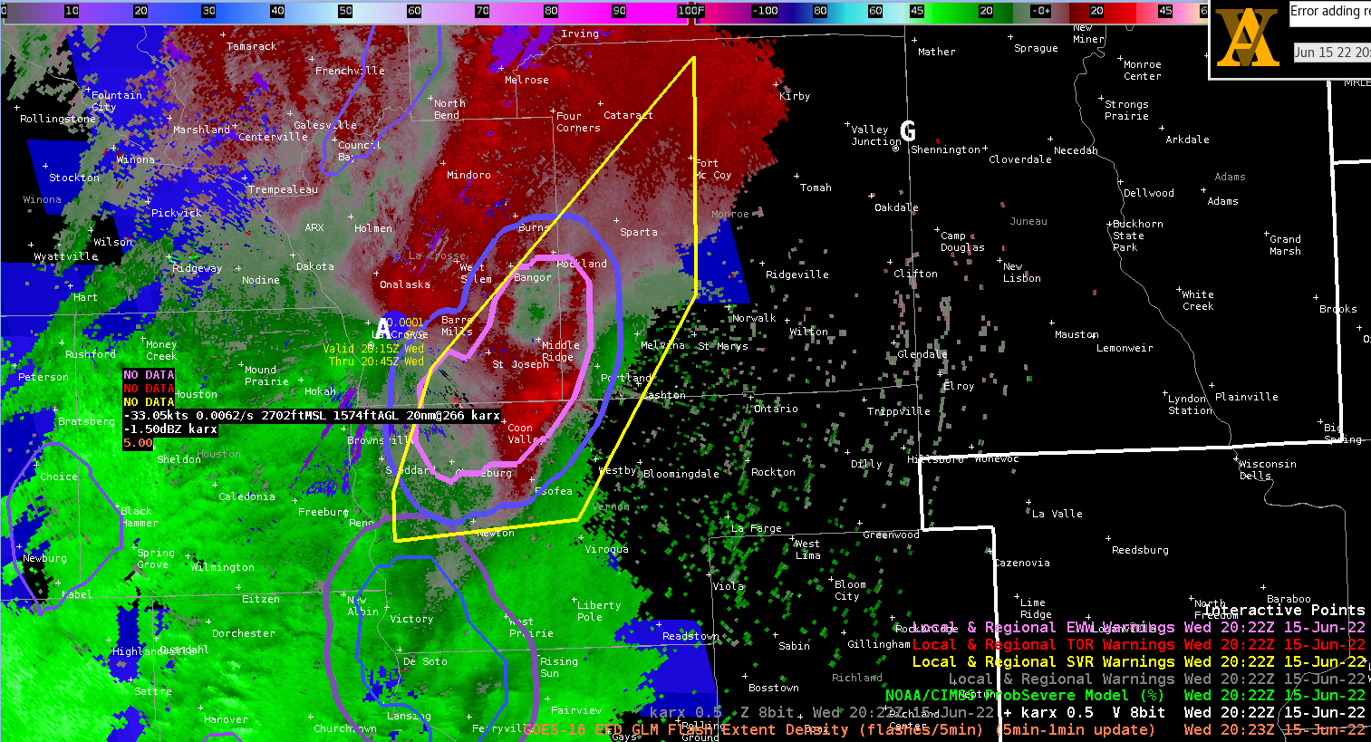
A user can also overlay lower layer wind fields to see what could be happening in those areas.  The key thing was though to see what the storm-top divergence may look like:

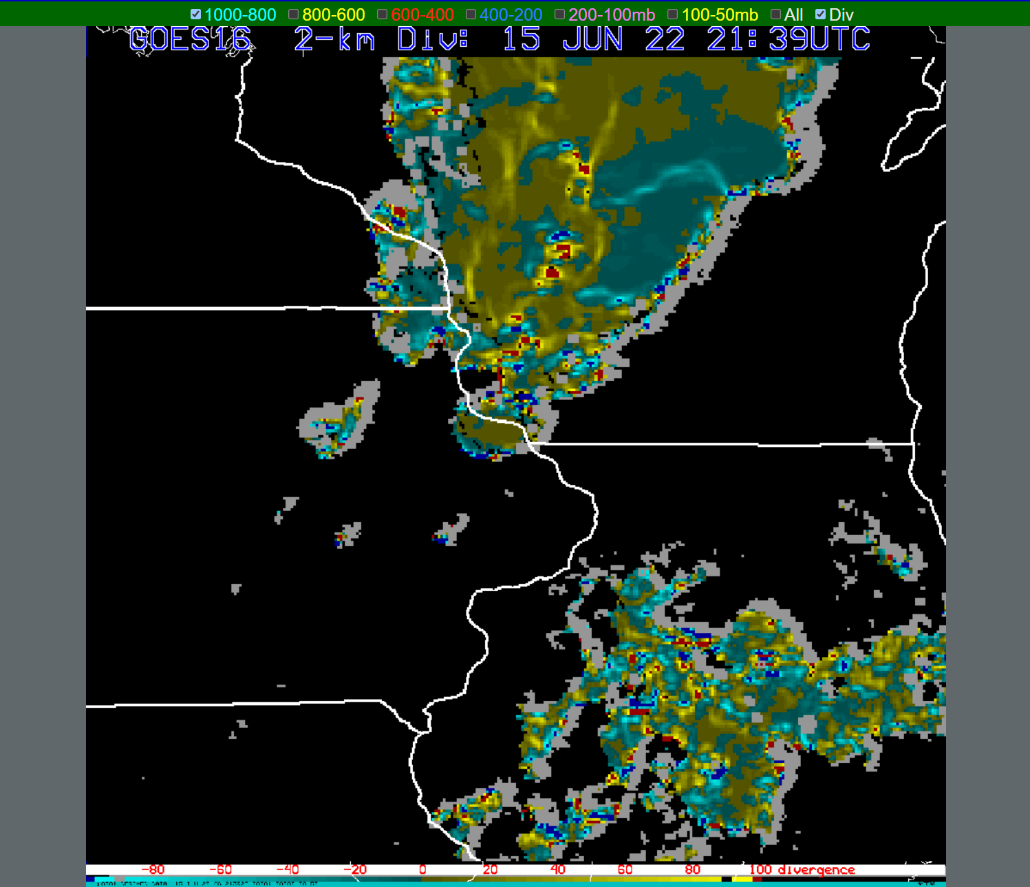
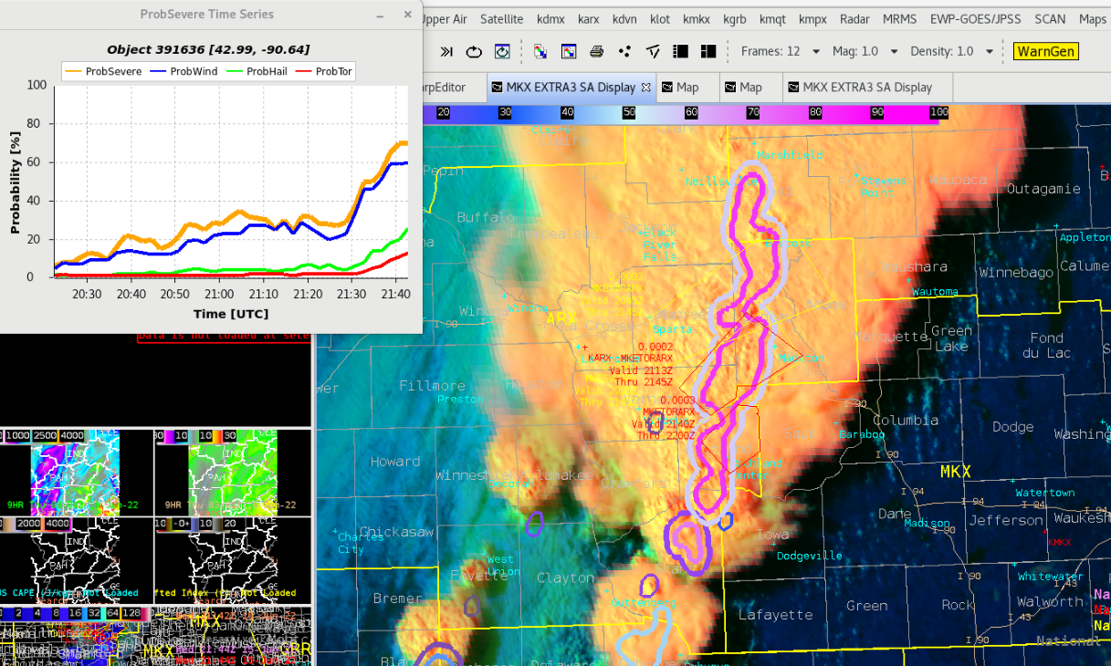
And that’s pretty impressive for an optically derived wind field!  Individual turrets may be showing up where there are enhanced area of convergence/divergence couplets not the ones on the edge of the cloud detection).  It isn’t perfect though:

There is a lot of variability from scan to scan on the strength of the divergence field but there is enough of a signal to figure out where the strongest couplets could be and which storm tops they could be associated with.  We couldn’t overlay radar data or the 3.9 micron “Red/visible” channel with a divergence product to make a 1:1 comparison; something to consider would be a grid that could be overlaid on a different ABI image to do a visual comparison to this product.

I’m impressed!

– Hank Pym

Pre-Convective Environment Across GRB

With a busy day still underway across Wisconsin, the use of the Optical Flow Winds, GLM, Prob Severe, and NUCAPS soundings were a big help in looking at the pre-convective storm environment and in warning operations.

When it came to looking at sounding data we had a NOAA-20, and AQUA pass for the polar orbiting satellites, that we could then compare to the special observed sounding from GRB.

There are some spatial differences in the locations since each satellite doesn’t pass over the exact location and the observed sounding came from the GRB office. I ended up grabbing NUCAPS soundings from west of the office where I thought the better storm environment would be. Regardless of this they do show great information over a temporal and spatial scale.
Just between Aqua (bottom image) and NOAA-20 (middle image) you can see that the environment becomes much more moist over time (AQUA came around 19Z and NOAA-20 came around 18Z). The increase in temperatures and dew points in the low levels between the two NUCAPS soundings show that there was increasing low level lapse rates and increasing CAPE through time. Then compare both of these to the special sounding sent out by GRB, you can see AQUAs vast improvement in the low level over NOAA-20. The one caveat seems to be the smoothing of the values in the mid levels. Smoothing seems to have decreased the values almost too much for both satellite soundings. It is fairly within reason given that there is a dry layer in the mid levels on the observed, but the smoothing looks to have slightly overdone it.
Moving on to the GLM, it was very helpful when boosting confidence in the warning operations. There were lightning spikes collocated with increasing rotation and reflectivity. The one things worth mentioning is to have a reminder or maybe even have offices lower/change the color curves for FED prior to the start of an event. It could even be a permanent change that some offices make.
Since I was the only one in the group to check, compare, and lower the FED color curve accordingly it was much easier to pick out lightning jumps. From the graphic above alone, 0-65 was much more informative than 0-128 or 0-260.
The last thing worth mentioning for the day was the Optical Flow Winds. While this was helpful in a warning environment to look at storm top divergence and speed of the winds at the tops of clouds, I was able to find another great use for it. In the pre convective environment I had pulled up the Optical Flow Winds and noticed that it was tracking winds and speeds of clouds over Lake Michigan. In an area where any wind information and observation data can be very sparse to near non-existent. The optical flow winds could be very helpful for open waters forecasting.
-Cirrus Fields

PHS Tornado Parameter

Unfortunately I didn’t look at this PHS Significant Tornado Parameter in real time when warnings were being issued, just completely spaced it.  But went back to see how it fared during the Tornado Warnings, it didn’t do too bad.  The comparison below is from 21z and even though the tornado warning was already issued before the PHS STP was available, it was a nice “confirmation” tool of the Tornado Warning.  The units of the STP were nearly 10 at the time of the strong couplet north of Clifton, WI and it was in the right location at the time of warning.

Figure 1: base reflectivity with ProbSevere Tor Model and warnings in effect.

Figure 2: base velocity animation of the strong couplet over Oakdale or just north of Clifton, WI.

Figure 3: PHS Significant Tornado Parameter at 21z on June 15, 2022. The circle over Clifton is a reference point for the velocity animation from Figure 2.

– PODIUM

NUCAPS Sounding Verification – Day 3 (June 15, 2022)

I had a great opportunity to get some verification on a NUCAP sounding that passed through shortly after 19z on June 15, 2022.  It was the NOAA-20 which just happened to pass over eastern Iowa where the DVN WFO launched a special sounding at 19z on the same day.  I’d estimate the locations of the two soundings compared were roughly 50-60 miles apart. The DVN sounding was equidistant from 4 NUCAP soundings and all those soundings had very similar readouts from one another (see Figure 1).  One of the disadvantages of the NUCAP soundings is no winds are measured, but there are plenty of other parameters that could be compared from the two soundings. The first thing that I compared were the CAPE values (See Table 1).  The other two tables below compare other various parameters.

Some interesting differences between the CAPE values measured. Uncertain why the NUCAP sounding doesn’t suggest any 0-3CAPE values, especially since the much larger surface based CAPE.  Another big difference that really stood out was the freezing level heights and the Convective Temperature. Obviously the NUCAP sounding may have overestimated the temperature profile and thus larger CAPE values, but I found it interesting that the freezing level from the NUCAPs sounding was slightly lower. The RH values were fairly similar, particularly the midRH values, but also eyeballing the dew point temperature profile, they are pretty close near the surface.

Overall, I do like the NUCAP soundings availability as it is another tool available for the forecast toolbox.  It might be wise (as with all things meteorology) to be careful with totally believing some of the NUCAP sounding readings after seeing this comparison.

Table 1: CAPE parameters compared from 19z soundings.  (J/kg)


Table 2: Comparing various parameters found in soundings. Note: LCL, LFC, LI, etc are all measured from the surface.


Table 3: Comparing various lapse rates and -20C/-30C heights.


Figure 1: Location of the DVN 19z special sounding and the NUCAPS NOAA-20 1921z sounding.

Figure 2: DVN special sounding launched at 19z on Jun 15, 2022.

Figure 3: NUCAP NOAA-20 sounding at 1943z on Jun 15, 2022.

– PODIUM

GLM Parallax and Lightning Cast Fun

The GLM data, specifically the FED data, was used to provide DSS to the Riverfest in La Crosse, WI.  After my first contact with the event POC, I noticed that the FED data was off by roughly a county from the ground-based lightning data.  This was my first time witnessing the parallax issue from the GLM and why ground-based lightning networks are a key component in confirming that the GLM location is accurate. In Figure 1, notice the intense concentration of the lightning just southwest of the event (20 mile and 5 mile radius rings) depicted by the GLM while the ENTLN/NLDN say that concentration is about a county south.   The parallax is evident in other lightning concentrations in and around the event circle.  I know it’s something being worked on to have the GLM data corrected to avoid this parallax issue, but it would be nice to have a map of the locations where the parallax is more evident in case you may not need the corrected version. Obviously, the further north, the larger the parallax, but not quite sure at what latitudes it really starts to show its hand. On a side note, for aviation purposes, the parallax could become problematic if the GLM lightning data is off by a factor of a county or two, especially if re-routing aircraft is occurring.

Figure 1: GLM Flash Extent Density compared with ENTLN data on June 15, 2022.

Figure 2: FED and ENTLN animation showing the GLM parallax.

I utilized the Lightning Cast to provide a probable end time of the lightning threat for the Riverfest event in La Crosse, WI.  This was a valuable tool as it provided some added confidence when the storms would exit the event area.  I did my best to line up the TOA tool with the 25 percentile contour. Once I got my estimated time that the end of the lightning threat would reach the event, then I added about 30 minutes to ensure it was well east of the event circle.

– PODIUM

Can PHS Improve Mesoanalysis and Near Term Convective Forecasts?

A large portion of the MKX CWA was included in a MDT severe risk, so by the start of the operational period, we had to assess the evolving severe threat spreading in from the west. Meanwhile, our DSS event was the Madison Jazz Festival, which entailed a focus specifically on south central Wisconsin. The PHS CAPE forecast appeared to be a noteworthy improvement from the CAPE fields on the SPC Mesoanalysis, along with the short-term forecast on that page.

Below are the 18z through 20z plots of MUCAPE, MUCIN and effective bulk shear from the SPC Mesoanalysis page.

Compare the above images with 4000 J/kg of uncapped MUCAPE to the PHS MUCAPE initialization at 18z and 2-hour forecasts (19z and 20z) below.

As you can see, while the SPC mesoanalysis was indicating 4,000 J/kg of uncapped MUCAPE, the PHS forecast showed CAPE decreasing across central and south central Wisconsin. This was an important and helpful piece of information for our DSS content for the Madison Jazz Festival.

The Day Cloud Phase RGB images below back up the PHS forecast vs the SPC mesoanalysis, as relatively flat Cu field over our area of interest actually dissipated between 20z and 22z.

Based on the PHS forecast combined with satellite analysis, we were able to focus the convective threat for the Madison area toward 6PM and onward, tied to the stronger forcing and better moisture arriving from the west where the ongoing convection resided closer to the cold front. It appears that the PHS sampling of moisture in the column applied to the near-term forecast strongly outperformed the SPC/RAP Mesoanalysis model background and OA algorithm.

Differences between the LightningCast (LC) CONUS and LC Mesos

Note below the CONUS scale (1st image) and Mesos (Meso Sector 2 on 6/15) had a different depiction of the lightning probability over northeast Iowa at 1911z 22Jun15. This was due to the time for a CONUS GOES-East scan to complete, vs. the much shorter time for a Meso sector, which in turn affects the LightningCast model. This is something to keep in mind when using the product.

ProbSevereV3 Trends for Severe Convection in Western/Southwestern Wisconsin

At 2106z, the ARX office had recently issued a Tornado Warning (2102z) for the northern cell with a high % on PSV3 and PTV3, per the noted superior calibration of the updated model vs. the V2. Could the PSV3 and PTV3 trend on this storm have assisted the radar operator in an increased lead time? As you can see below, starting at 2045z, there was a sharp upward trend in the ProbTor, to near 40% prior to 21z. At the least, this tool appears to be an excellent situational awareness tool, and may even be able to help lead time in some cases. It helped us in the MKX CWA regarding downstream warning issuances. In the event of an unexpected radar outage in a sparse radar coverage area, environmental analysis plus satellite interrogation with the utility of PSv3 could support successful radar warning ops in a less than ideal scenario.

– Hurricane84

Situational Awareness and Lead Time with LightningCast and ProbSevere/Tor

Today’s experience landed us in MKX monitoring convective development potential across the western portion of the CWA, with a line of storms ultimately moving in from the west, and some risk of discrete cells persisting even after we ceased the experiment.

I took the opportunity today to set up procedures overlaying PHSnABI indices (CAPE) with satellite imagery (e.g. Day/Cloud Phase or Viz), to see how well it corresponded with convective development. Unfortunately I didn’t grab a screenshot, but it was a nifty display that I hope to use again. PHSnABI suggested that CAPE in some areas of the CWA was not as high as the SPC mesoanalysis or RAP suggested. We tried to investigate this using a combination of NUCAPS and model soundings and RAOB, but couldn’t figure out a reason for the CAPE depression before incoming storms grabbed our attention. Notably, the indices derived only from GOES agreed with PHSnABI about this depression, though we couldn’t figure out if it was correct. It seems likely the GOES ABI was driving the PHSnABI result.

My main takeaway the rest of today is how useful ProbSever, ProbTor, and LightningCast can be with approaching/developing convection.

LightningCast, combined with GLM data, was useful for IDSS imagery to depict position and potential of lightning (example DSS slide using these graphics provided below).  Storms never made it to our decision point prior to leaving the experiment, but lightning threat was usefully communicated to the simulated JazzFest event.

As convection developed, we also practiced relying on probSevere and probTor for lead time in anticipating warnings. The following shows an example where the probTor trends corresponded well with ARX’s actual decision to issue a tornado warning.

SImilarly, intensification of the convective line appeared to be well detected. In fact, depending on what threshold of the probSevere parameters is relied on (probably depends on environment and other factors), the escalating value could have given useful lead time for a severe issuance decision.

Although the main mode appeared to be a line of convection, there were positions along the line where tornado risk seemed to increase (evidenced by radar velocity). It was reassuring to see probTor pick up on the gradually increasing risk of tornadoes as well.

And one final note… lightningCast is fairly impressive in how it produces calibrated estimates of lightning occurrence using only a single time step of satellite imagery (though it uses several bands of the ABI). Naturally lightningCast has difficulty where a developing tower is obscured by an anvil overhead, as we saw in this example. But it was neat to see lightningCast immediately respond with a broader swath of high lightning probabilities the very first time that a tower poked above the anvil that previously obscured it.  The fact that it was hidden probably means lightning could have been occurring below the anvil with lower than ideal lightningCast probabilities (though non-zero, to its credit), but it was neat to see the immediate adjustment to the probability contours with new imagery.

– Buzz Lightyear

ProbSvr V3 ProbTor

The LaCrosse office was busy today with multiple storms that exhibited rotation. ProbSvr/ProbTor was helpful in the case of situational awareness and triaging the storms. Below is an example of a case where ProbTor decreased significantly over a period of a few minutes. In this case, ProTor slowly increases over a 10-15 minutes as the storm exhibits some rotation. A lightning jump was also noted with the peak probabilities of ProbTor around 40% at 2016 UTC. All of the parameters decrease significantly over a 5-6 minute period of time by 2022 UTC (images of reflectivity and velocity are included below). The lightning decreases dramatically as seen in the chart below as does the azimuthal shear (based on the chart and 0.5 velocity). A severe was already out for this storm and ProbSvr remained high throughout much of the lifecycle of the storm. As the warning forecaster, it was nice to see the confirmation of the lower probabilities. A severe warning was already out and the storm was covered for those threats. It was nice to have the confirmation from ProbTor to turn my attention to other storms that may need a warning or be on the verge of warning issuance.

2016 UTC 0.5 Reflectivity

2016 UTC 0.5 Velocity

2022 UTC 0.5 Reflectivity

2022 UTC 0.5 Velocity.

– Marty McFly

The utility of satellite derived data in mesoanalysis & near term convective forecasting

The most common mesoanalysis tool is the SPC (RAP) Mesoanalysis Page

While there was no new convection in the operational period for the RNK CWA, satellite based products did show their utility as a cross check with the SPC Mesoanalysis. Since the SPC Meso-a page starts with a RAP model background field, the ability to QC check this data will be helpful in gauging the accuracy of hourly RAP and HRRR model fields. In this way, you can gauge whether the Mesoanalysis and hourly updating fields are either on track or likely vary in meaningful ways from satellite derived data.   Having this data will be especially useful in locations that do not have frequent or any aircraft vapor soundings.

Mid-level lapse rates

SPC Meso-A 700-500 mb lapse rates at 19z 6/14

NUCAPS 700-500 mb lapse rates at 1819z 6/14

Excluding the likely unreliable data in the region of lingering cloud cover across central Virginia, the NUCAPS data roughly ranged from 6.5C to 7.6C/km across the RNK CWA, which is fairly close to the SPC Meso-A 700-500 mb lapse rates. Within the past few years, maximum 2-6 km AGL lapse rates were added to the SPC Meso-A page. The question I had was, with its good mid-level moisture sampling, would a NUCAPS sounding be a good QC check for the SPC max 2-6 km AGL LR field? Examples are shown below.

SPC Meso-A Max lapse rate (C/km) in 2-6 km AGL layer at 19z 6/14

NUCAPS sounding near Martinsville, VA at 1819z 6/14

As you can see from the SPC mesoanalysis graphic, there was a region of 7.5 C/km to 8.4 C/km maximum lapse rates in the 2-6 km AGL layer. The NUCAPS sounding above sampled a layer of 7.9 C/km lapse rates from just below 700 mb to just below 500 mb, which verifies the SPC Meso-A field.

CAPE analysis

SPC Meso-A SBCAPE and SBCIN at 20z 6/14

SPC Meso-A MLCAPE and MLCIN at 20z 6/14

SPC Meso-A MUCAPE and LPL at 20z 6/14

Here we’ll compare the SPC Meso-A graphics to the PHS initialization at the same hour.

PHS SFC CAPE at 20z 6/14

In general, the CAPE values on the satellite derived initialization is less aggressive the SPC Meso-A SBCAPE, but the distribution is similar, showing a west to east gradient, with lower values east where there remained lingering debris cloud cover. The MLCAPE and MUCAPE fields show a similar west-east gradient in CAPE, while SBCIN and MLCIN are also maximized in the cloud cover area across central VA.

The gridded NUCAPS MAXCAPE field was from the 18z hour per 1819z sounding availability, and was noisier data as would be expected due to unreliable retrievals under thick cloud cover.

Gridded NUCAPS MAXCAPE at 18z 6/14

Excluding the bullseye to the northeast, the distribution on the NUCAPS compares favorably to the SPC Meso-A MUCAPE field. Furthermore, recalling the NUCAPS 1819z sounding near Martinsville, MUCAPE values over that area on the SPC Meso-A field vs. the NUCAPS sounding match up well. While the time difference between the NUCAPS and SPC Meso-A fields is something to take into consideration when using the data, the less than 2-hour difference between them helps in this case. Furthermore, if we were using the NUCAPS data to compare to the SPC Meso-A graphics, we would’ve done a direct 18z check as well.

– Hurricane84

A Close Look at LightningCast for the Application of DSS or TAF Support

On June 15th 2022, a dynamic setup was unfolding across Iowa, Minnesota, and Wisconsin with multiple hazards that NWS forecasters would have had to message and warn. For this case, we were on watch for a DSS event representing the Cranberry Blossom Festival in Wisconsin Rapids in the GRB CWA. The main concerns with the event were lightning and any severe storms, both of which seemed certain for this case and the name of the game was timing the oncoming convection.

LightningCast uses machine learning with numerous satellite inputs that yields the probability of lightning occurring at a location within the next hour. This product immediately jumps to the front of a forecaster’s mind to apply for decision support services (DSS) or assessing lightning probability for airport forecasting. Below is a table showing the probabilities from LightningCast versus the “time of arrival” tool that estimated storm timing based on the movement of storms:

First vicinity lightning strikes (within 10 mi of event): 4:21 PM
Arrival of storms (within 10 mi of event): 4:30 PM
Immediately the usability of this product is fantastic. It shows the probabilities of lightning occurring in a contour format, making it a great pairing with satellite imagery, lightning data, and radar. WIth this case being a very well forced event the main evaluation was the percentages and how they did with the advection of the storms. The LightningCast seemed to ebb and flow with the eastward acceleration and deceleration of the storms between 3 and 3:30 PM, while the next 15 minutes showed accelerating storms, giving a 61% chance of lightning within the next hour at 3:45 PM. With the acceleration of the storms, it was good to see the model adjust, with the 50% threshold being crossed before 3:45 PM. The 50% threshold is very important for forecasters, as values above that are typically  used in several products and gauges of confidence. The LightningCast model giving upwards of 40 minutes of lead time for advecting storms gives me a lot of confidence in the product, leaving me wishing it was already available within our datasets for immediate use.
– aerobeaver