This is the initial “welcome” post for the Lightning Jump Algorithm test. Please come back using the direct link to the “Lightning Jump Algorithm” category for additional posts.
Greg Stumpf, CIMMS/MDL
Official websites use .gov
A
.gov website belongs to an official government
organization in the United States.
Secure .gov websites use HTTPS
A
lock (
) or https:// means you’ve safely connected to
the .gov website. Share sensitive information only on official,
secure websites.

This is the initial “welcome” post for the Lightning Jump Algorithm test. Please come back using the direct link to the “Lightning Jump Algorithm” category for additional posts.
Greg Stumpf, CIMMS/MDL
For my presentation at the 2011 NWA Annual Meeting in Birmingham, I wanted to introduce the concept of geospatial warning verification and then apply it to a new warning methodology, namely Threats-In-Motion (TIM). To best illustrate the concept of TIM, I’ve been using the scenario of a long-track isolated storm. To run some verification numbers, I needed a real life case, so I chose the Tuscaloosa-Birmingham Alabama long-track tornadic supercell from 27 April 2011 (hereafter, the “TCL storm”), shown in earlier blog posts, and I’ll repeat some of the figures and statistics for comparison. This storm produced two long-tracked tornadoes within Birmingham’s County Warning Area (CWA).
The choice of that storm is not meant to be controversial. After all, the local WFO did a tremendous job with warning operations, given the tools and they had and within the confines of NWS warning policy and directives. Recall the statistics from the NWS Performance Management site:
Probability Of Detection = 1.00
False Alarm Ratio = 0.00
Critical Success Index = 1.00
Percent Event Warned = 0.99
Average Lead Time = 22.1 minutes
These numbers are all well-above the national average. We then compared these numbers to those found using the geospatial verification methodology for “truth events”:
CSI = 0.1971
HSS = 0.2933
Average Lead Time (lt) = 22.9 minutes
Average Departure Time (dt) = 15.2 minutes
Average False Time (ft) = 39.8 minutes
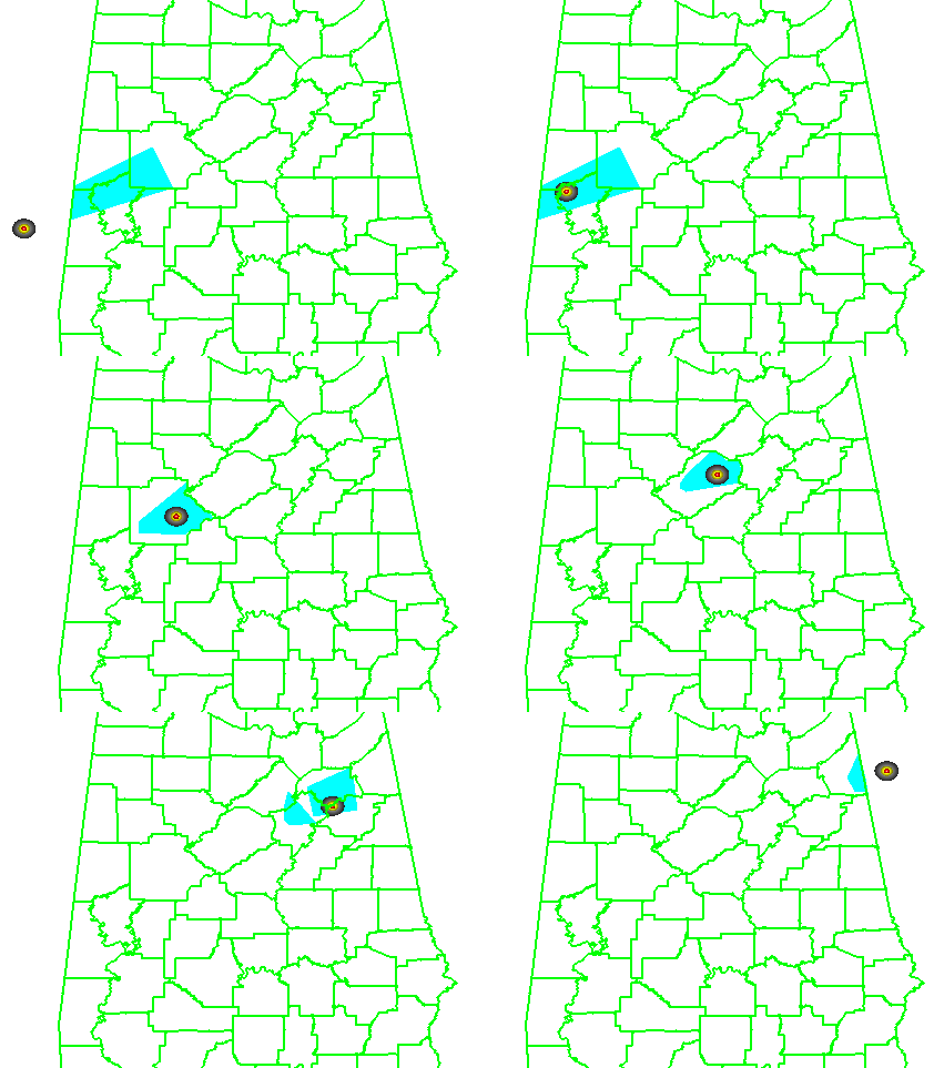
And recall the animation of the NWS warnings I provided in an earlier blog post:
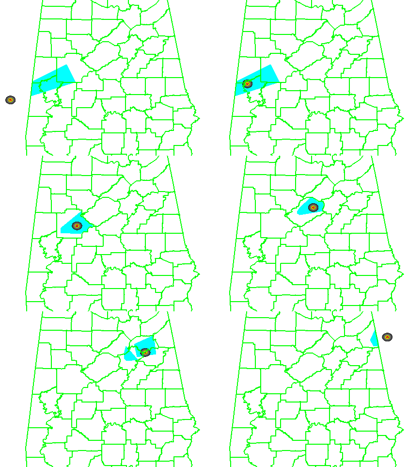
What if we were to apply the Threats-In-Motion (TIM) technique to this event? Recall from this blog entry that I had developed a system that could automatically place the default WarnGen polygons at the locations of human-generated mesocyclone centroids starting at the same minute that the WFO issued its first Tornado Warning on the storm as it was entering Alabama. I used a re-warning interval of 60 minutes. If you adjust the re-warning interval to one minute (the same temporal resolution of the verification grids), you now have a polygon that moves with the threat, or TIM. The animation:
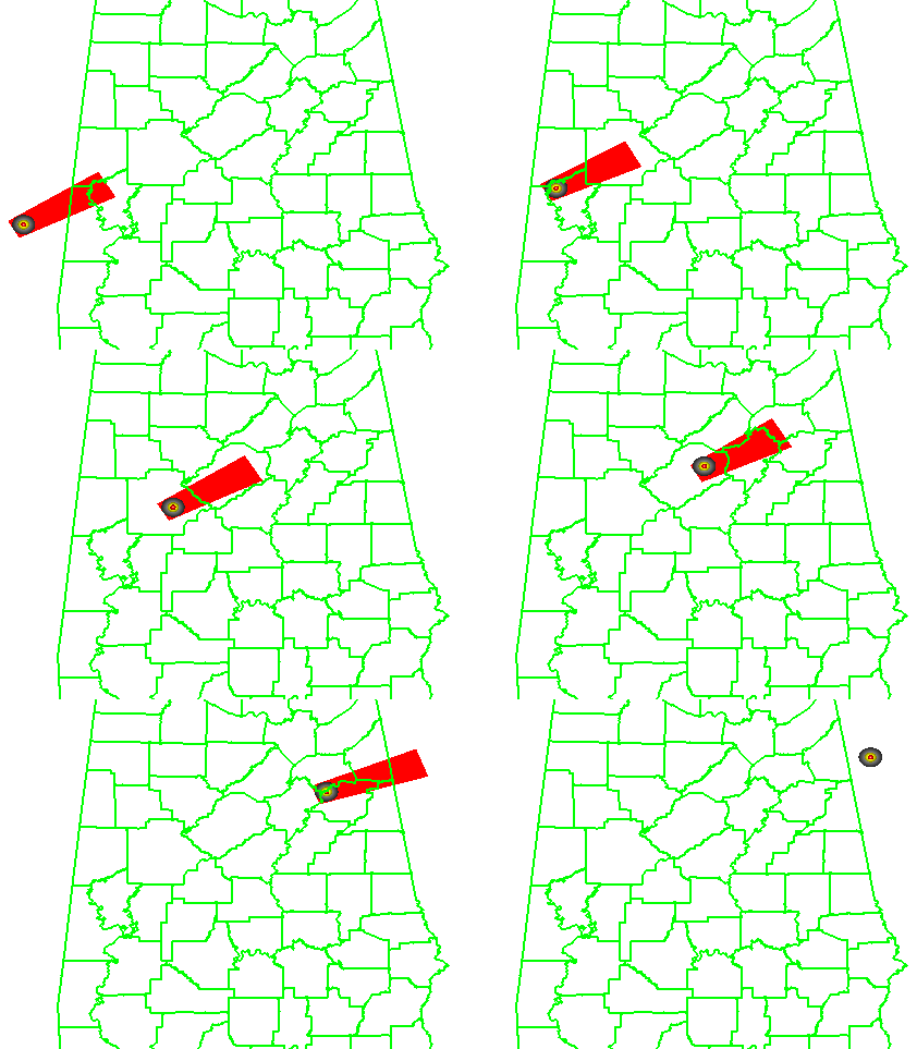
Let’s look at the verification numbers for the TIM warnings:
CSI = 0.2345
HSS = 0.3493
Average Lead Time (lt) = 51.2 minutes
Average Departure Time (dt) = 0.8 minutes
Average False Time (ft) = 23.1 minutes
Comparing the values between the NWS warnings and the TIM warnings visually on a bar graph:
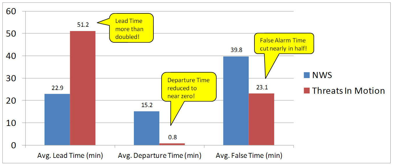
All of these numbers point to a remarkable improvement using the Threats-In-Motion concept of translating the warning polygons with the storm, a truly storm-based warning paradigm. Let’s also take a look at how these values are distributed in several ways. First, let’s examine Lead Time. The average values for all grid points impacted by the tornado (plus the 5 km “splat”) are more than doubled for the TIM warnings. How are these values distributed on a histogram:


For the TIM polygons, there are a lot more values of Lead Time above 40 minutes. How do these compare geospatially?
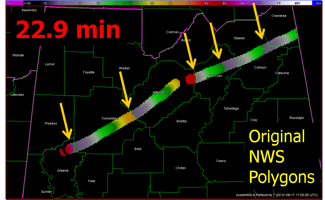
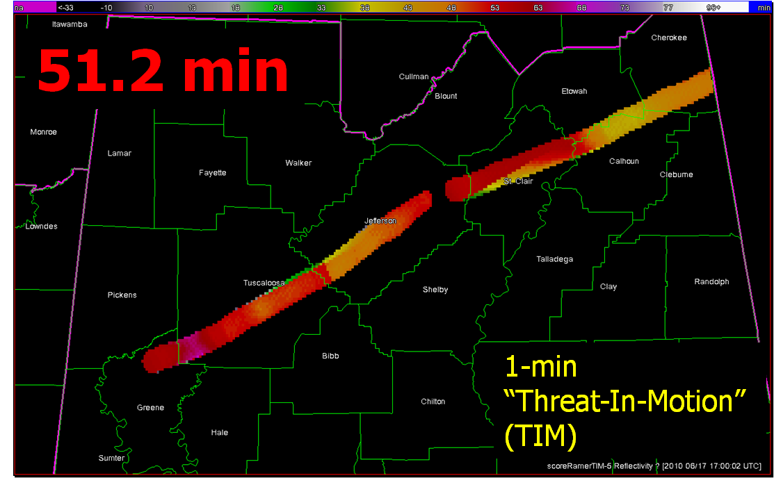
Note that the sharp discontinuities of Lead Time (from nearly zero minutes to over 40 minutes) at the downstream edges of the NWS warnings (indicated by yellow arrows in the top figure) are virtually eliminated with the TIM warnings. You do see a few discontinuities with TIM; these small differences are caused by changes in the storm motions at those warned times.
Moving on to Departure Time, the average values for all grid points impacted by the tornado (plus the 5 km “splat”) are reduced to nearly zero for the TIM warnings. How are these values distributed on a histogram:


And geospatially:
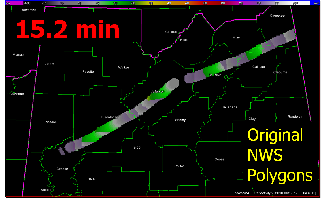
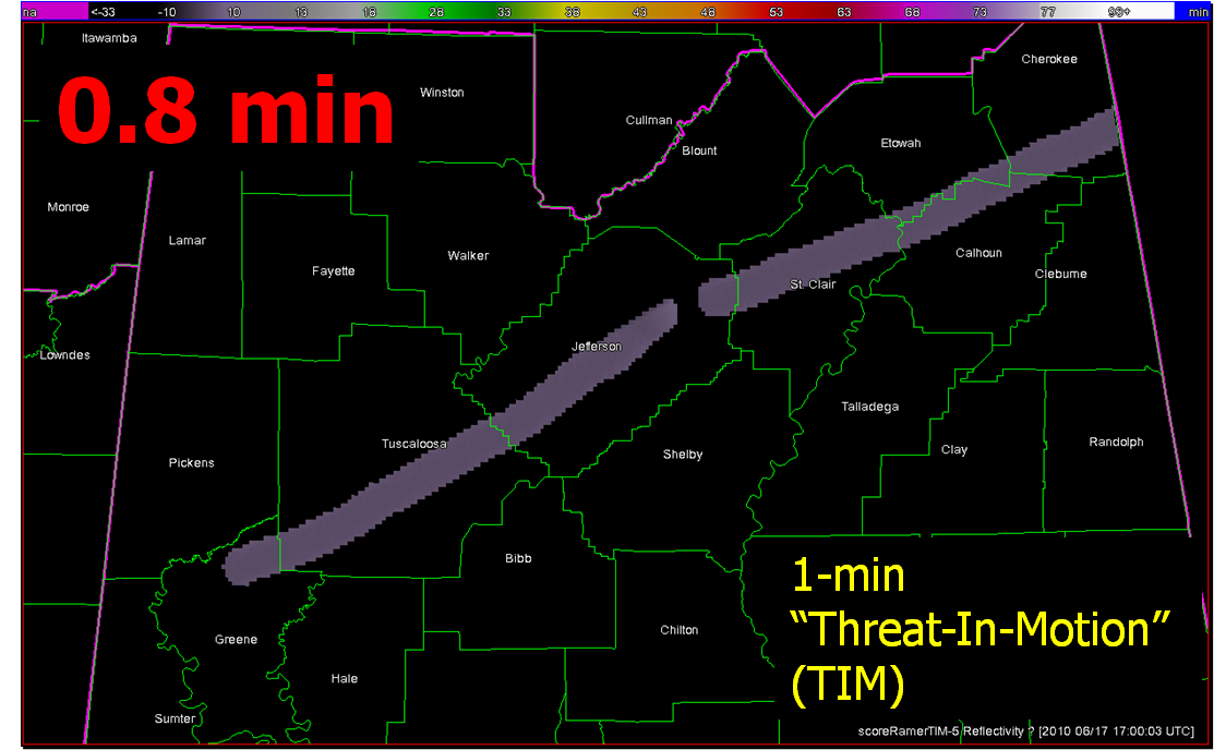
With the TIM polygons, the departure times across the path length of both tornadoes is pretty much less than 3 minutes everywhere. Whereas, the NWS polygon Departure Times are much greater, and there are some areas still under the NWS warning more than 30 minutes after the threat had passed.
Finally, looking at False Alarm Time distributions both on histograms and geospatially:


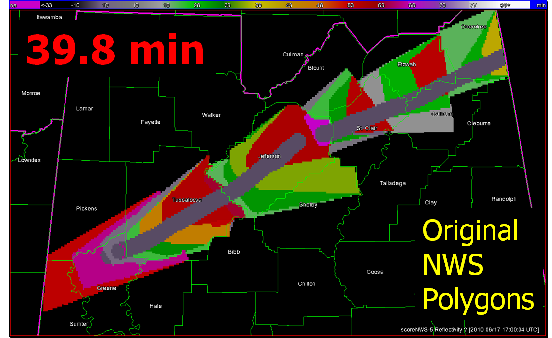
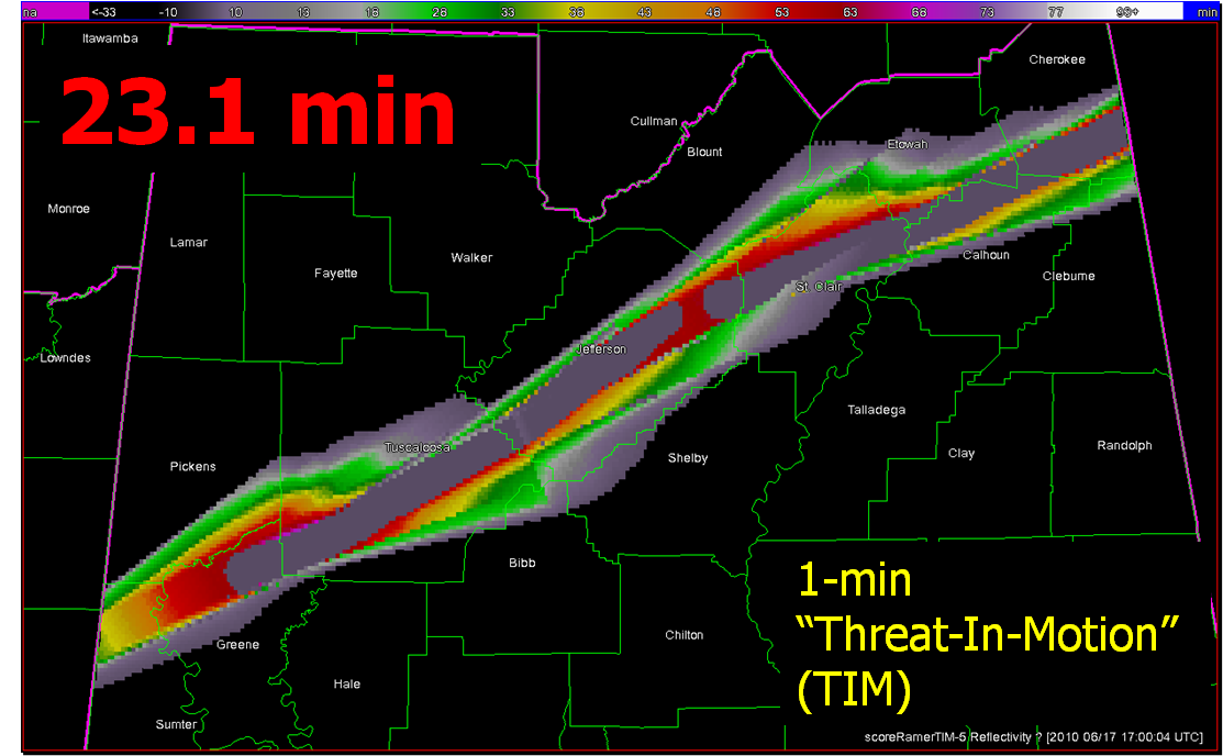
There are some pretty large areas within the NWS polygons that are under false alarm for over 50 minutes at a time, even though these warnings verified “perfectly”. In comparison, the TIM warnings have a much smaller average false alarm times for areas outside the tornado path (about a 42% reduction). However, there are a number of grid points that are affected by the moving polygons for just a few minutes. How would we communicate a warning that is issued and then canceled just a few minutes later? That is food for future thought. I’ve also calculated an additional metric, the False Alarm Area (FAA), the number of grid points (1 km2) that were warned falsely. Comparing the two:
NWS FAA = 10,304 km2
TIM FAA = 8,103 km2
There is a 21% reduction in false alarm area with the TIM warnings, much less than the reduction in false alarm time. The reduction in false alarm area is more a function in the size of the warning polygons. The WarnGen defaults were used for our TIM polygons, but it appears that the NWS polygons were made a little larger than the defaults.
So, for this one spectacular long-tracked isolated supercell case, the TIM method shows tremendous improvement in many areas. But there are still some unanswered questions:
Future blog entries will tackle these.
Greg Stumpf, CIMMS and NWS/MDL
Here I’m going to describe the “Threats-In-Motion”, or TIM concept that was presented at the 2011 National Weather Association Annual meeting. Essentially, once a digital warning grid is created using the methodology presented in the previous blog entry, the integrated swath product would start to translate automatically. The result would be that the leading edge of the polygon would inch downstream, and the trailing edge would automatically clear from areas behind the threat. We hypothesize that this would result in a larger average lead time for users downstream, which is desired. In addition, the departure time of the warning should approach zero, which is also considered ideal. The concept is first illustrated with a single isolated long-tracked storm for ease of understanding. Later, I will tackle how this will work with multi-cell storms, line storms, and storms in weak steering flow.
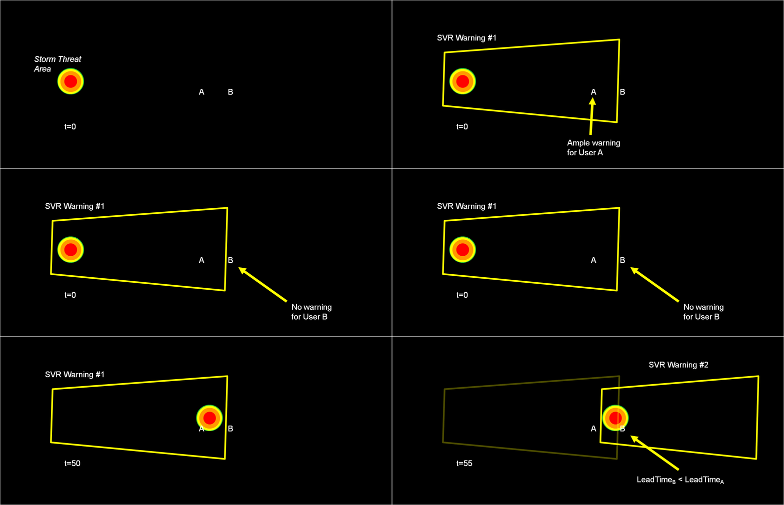
Why are Threats-In-Motion desired? Let’s look at the way most warning polygons are issued today. Threats that last longer than the duration of their first warning polygon will require a subsequent warning(s). Typically, the new warning polygon is issued as the current threat approaches the downstream end of its present polygon or when the present polygon is nearing expiration. This loop illustrates this effect on users at two locations, A and B. Note that only User A is covered by the first warning polygon (#1), even though its location is pretty close to User B’s location. Note too that User A gets a lot of lead time, about 45 minutes in this scenario. When the subsequent warning polygon (#2) is issued, User B is finally warned. However, User B’s lead time is only a few minutes, much less than User A who may only live a few miles away.
What if a storm changes direction or speed. how are the warnings handled today. Warning polygon areas can be updated via a Severe Weather Statement (SVS), in which new information is conveyed and the polygon might be re-shaped to reflect the updated threat area. This practice is typically used to remove areas from where the threat already passed, thus decreasing departure time. However, NWS protocol disallows the addition of new areas to already-existing warnings. So, if a threat areas moves out its original polygon area, the only recourse is to issue a new warning, sometimes before the original warning has expired. You can see that in this scenario:
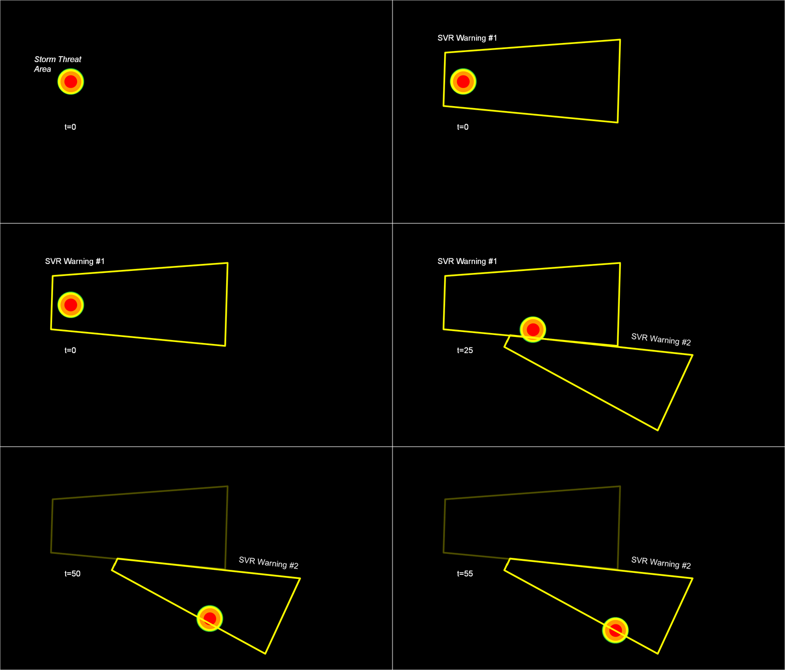
Note that a 3rd polygon is probably required at the end of the above loop too!
In the past entry, I introduced the notion of initial and intermediate forecasted threat areas. The forecasted areas can update rapidly (one-minute intervals), and the integration of all the forecast areas results in the polygon swath that we are familiar with today’s warnings. But, there is now underlying (digital) data that can be used to provide additional specific information for users. I will treat these in later blogs:
But what about “Threats-In-Motion” or TIM? Here goes…
Instead of issuing warning polygons piecemeal, one after another, which leads to inequitable lead and departure times for all locations downstream of the warning, we propose a methodology where the polygon continuously moves with the threat. Our scenario would now look like this:
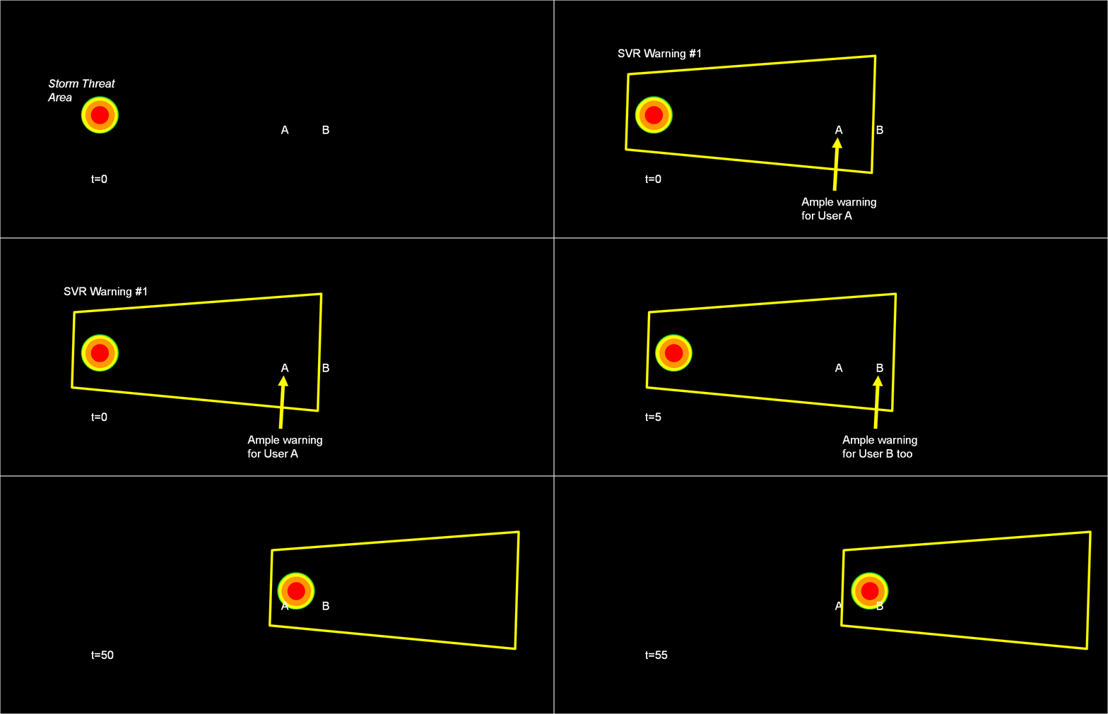
Note that User A and User B get equitable lead time. Also note that the warning area is cleared out continuously behind the threat areas with time. And here is the TIM concept illustrated on the storm that right turned.
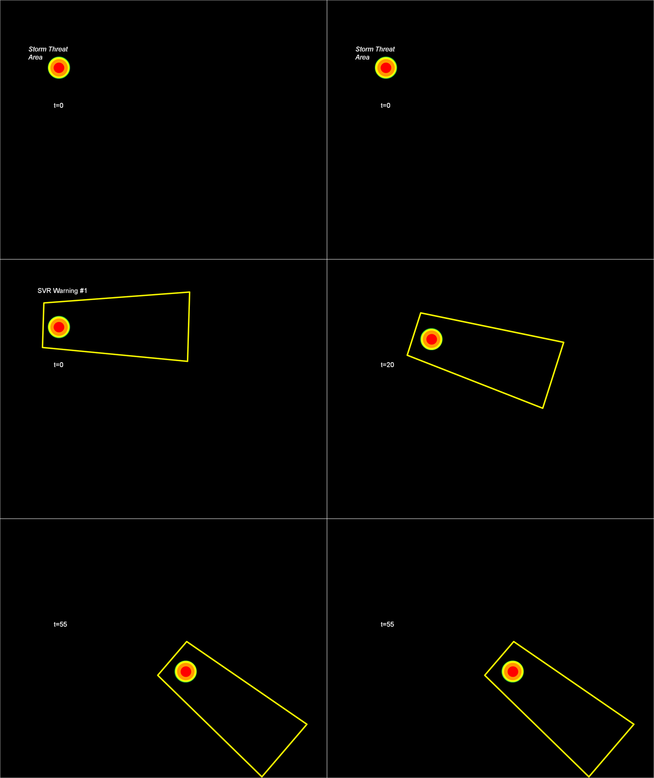
Now let’s test the hypotheses stated at the beginning of this entry. Does TIM improve the lead time and the departure time for all points downstream of the threat? If yes, what about the other verification scores introduced with the geospatial verification system, like POD, FAR, and CSI? The next blog entry will explore that.
Greg Stumpf, CIMMS and NWS/MDL
We will now introduce a new approach to creating convective weather hazard information which was first tested at the NOAA Hazardous Weather Testbed (HWT) with visiting NWS forecasters in 2007 and 2008. The new warning methodology varies in complexity and flexibility, but we will first present the basic concepts first. In this approach, the forecaster still determines a motion vector and chooses a warning duration. However, instead of tracking points and lines, the forecaster outlines the probable severe weather threat area at the current time, and inputs motion uncertainty. From this information are derived high-resolution rapidly-updating geospatial digital hazard grids. These grids are used to generate a wide variety of useful warning information, including warning swaths over a time period, meaningful information for time of arrival and departure for any location within the warned area, and probabilistic information based on the storm motion uncertainty.
First, let’s tackle the subject of this entry, “let’s get digital”. Right now, the official warning products are still transmitted as an ASCII text product, and all the pertinent numerical information in the warning like begin and end times, polygon lat/lon coordinates, and other information needs to be “parsed” out of the text product in order for various applications to take advantage of them (e.g., iNWS mobile alerting). This is an archaic method to deliver information, especially in this day and age of digital technology. Various options are being explored to improve the data delivery method, including encoding the warning information into the Common Alerting Protocol (CAP) format. While we feel this is an improvement, it is not going to be sufficient to completely convey all the possible modes of hazard information that can be created and delivered. For example, the polygon information is still encoded as a series of lat/lon points within the CAP formatted files. But what if the polygon is comprised of complex boundaries or curved edges? Or what if we want to include intermediate threat area information at specific times steps during the warning? Considering that we’ve made the argument for gridded warning verification, we feel that hazard information should be presented as a digital grid, more easily exploitable by today’s technology. You’ll understand why in a little bit…
So first addressing how a forecaster determines a current threat, instead of choosing points or lines and trying to decide where to place these points within the storm hazard areas, we feel that the warnings should be based on the tracking of a threat area. Here are the proposed steps in this new warning process. For each step, I’ve also added a snippet of ideas for “more sophistication” that I may explore further in later blog entries.
1. The forecaster outlines the current threat area.
For our HWT exercises, we gave the forecaster two options, a) draw a free-hand multi-sided polygon, or b) fit the current threat area with and ellipse. (The latter was offered because it is easier to project an area described by a known mathematical function, than it is for a free-hand polygon area). Where is the threat outline drawn? That is currently up to the forecaster to make their best determination where the severe weather currently resides in the storm. They can make use of radar and other data as well as algorithms for their decisions. Fig. 1 illustrates an initial threat area defined as a circular area. A circle is chosen to illustrate the effect of some of the later concepts below.
[More sophistication: The threat area is currently a deterministic contour (inside = yes or 100%, outside = no or 0%), but because we are entering data digitally, this initial threat area could be a probabilistic grid. For now, to keep it simple, we’ll just go with “you’re either in or you’re out”.]
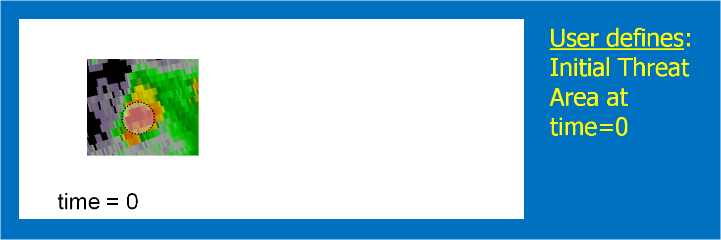
2. Determine the threat motion vector.
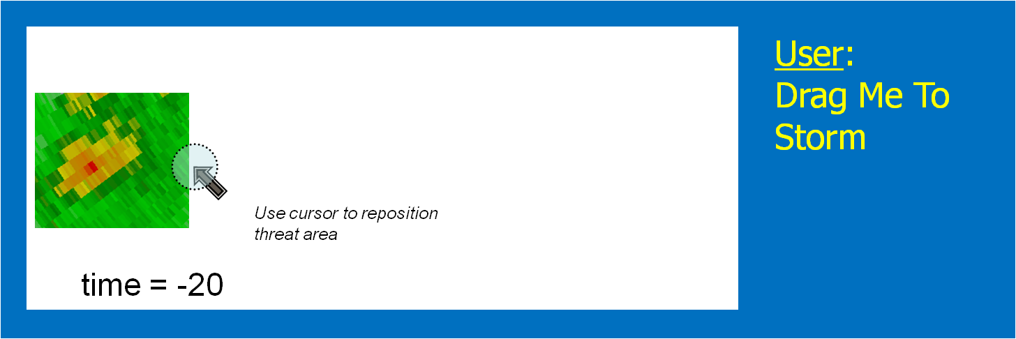
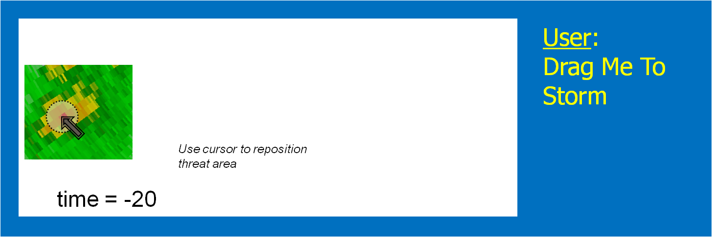
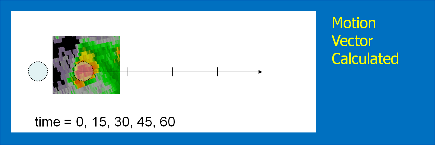
The motion vector could be determined using today’s WarnGen method of “Drag Me To Storm”. This is done by finding a representative location in the storm to track on the current radar volume scan, and then stepping back to a past volume scan (Fig. 2; 20 minutes in the past) and dragging the point to the same feature (Fig. 3). The distance and orientation between the current and past points would define the motion vector (Fig. 4). This is how we did it during our HWT exercises.
[More sophistication: Determine the motion vector by stepping the radar data back in time and repeating the process in step 1, drawing another threat hazard area. Then, an application such as the K-Means segmentation algorithm developed by NSSL could determine the motion vector betwen the two threat areas, or even a high-resolution two-dimensional motion field.]
3. Choose a warning duration.
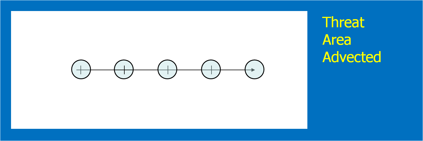
This is usually easy – how long does the forecaster want the warning to extend. The initial threat area is then projected to the final position. In addition, the threat area is projected to every time step between the warning issuance time and the warning duration time. We used a time interval of one minute in the HWT experiment. Figure 5 shows the projected threat area at 15-minute intervals; the intermediate intervals are not shown. Remember this aspect of the methodology! It has great implications, which I will explain soon.
[More sophistication: Typically, Severe Thunderstorm Warnings and Tornado Warnings rarely exceed 60 minutes, even if the forecaster is tracking a well-defined long-tracked supercell that has a high certainty of surviving past 60 minutes – simply due to NWS warning protocol. The warning duration could be “indefinite” until the hazard information blends upscale with information from nowcasts and forecasts. How? We’ll get to that later.]
4. Determine the uncertainty of the motion estimate.
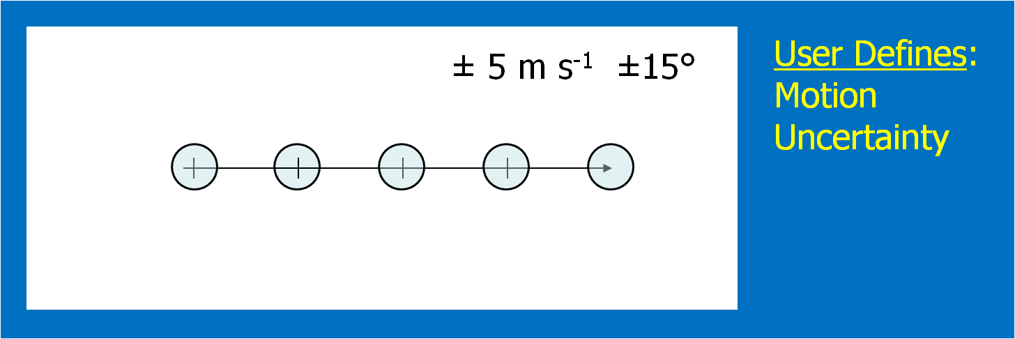
This could be approached in a number of different ways. For the HWT experiments, the forecasters simply chose a range of symmetric speed and direction offsets. For example, ±30° and ±5 kts. Although we didn’t offer this choice during the 2007-8 HWT experiments, the offsets could be asymmetric (e.g., + 30°, -10°, +5 kts, -8 kts). Fig. 6 shows an example offset for motion uncertainty. Figs. 7 and 8 show how speed and direction uncertainty (respectively) affect the shape of the translating initial threat area in time. Speed (direction) uncertainty stretches the initial threat area parallel (perpendicular) to the motion vector.
[More sophistication: The motion uncertainty could come from a theoretical model of storm motion behavior, such as Bunkers’ storm motion estimate for right-turning supercell thunderstorms, or a statistical model such as the Thunderstorm Environment Strike Probability Algorithm (THESPA) technique (Dance et al., 2010; see their Eq. 1).]
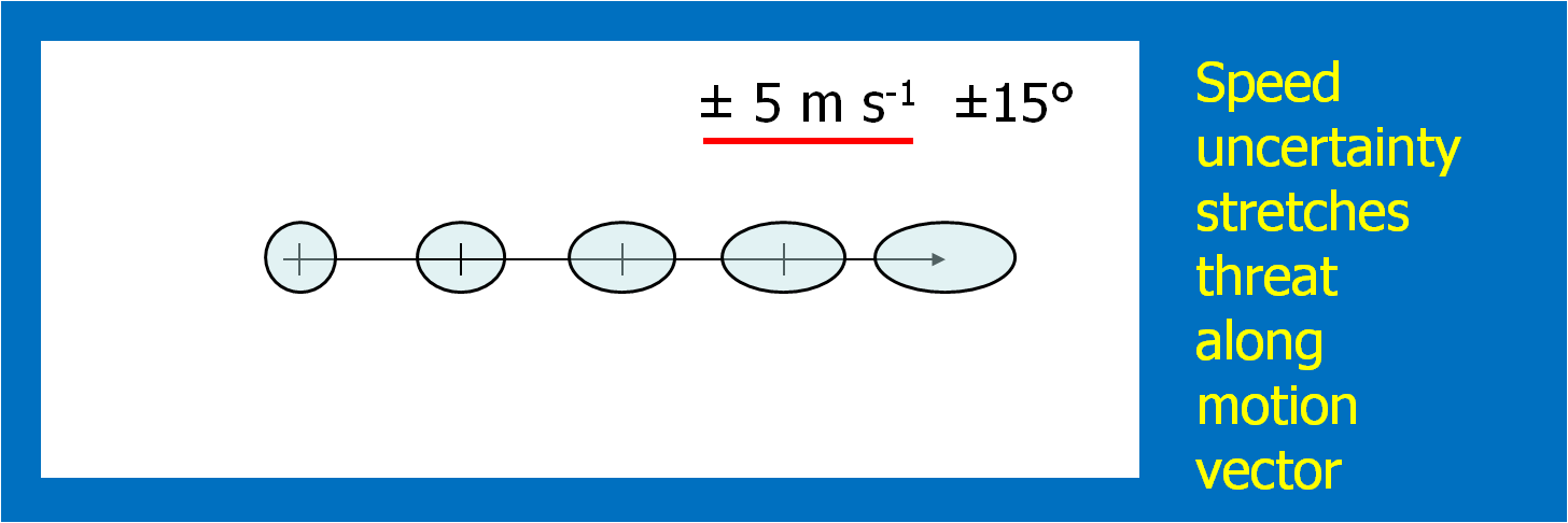
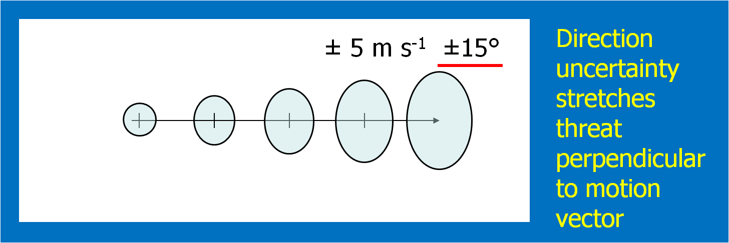
Once the above four quantities have been chosen by the forecaster, we can then generate a downstream “swath” that will be affected by the translating threat area. The swath is simply the total integration of all of the one-minute interval translating threat areas during the duration of the warning (Fig. 9).
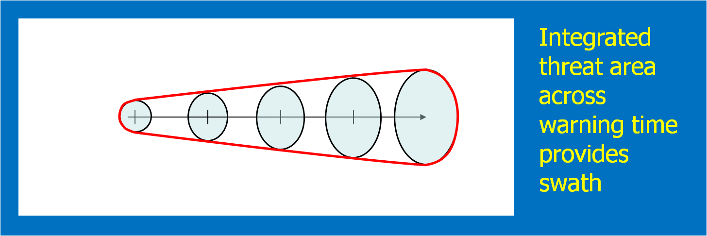
Here’s a better way to visualize the above static figure. Figure 10 shows a loop of the translating threat area over the forecast interval. The moving threat areas, integrated over the duration of the warning, providing the swath.
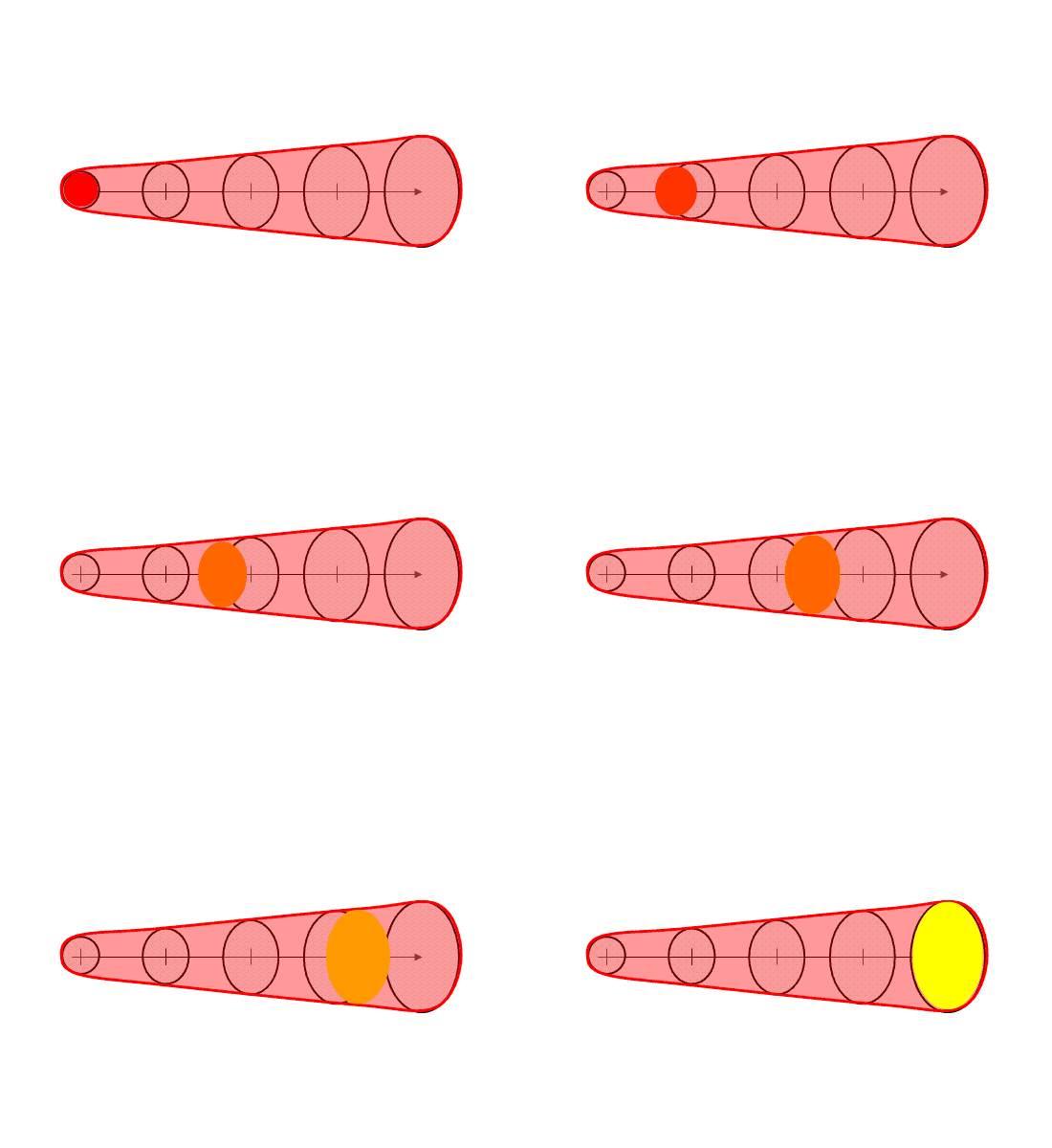
Note that the resulting “polygon” is exactly tied to the parameters of the warning as determined by the forecaster. The resulting integrated polygon cannot (and should not) be editable. The forecaster can only control the shape and position of the swath by changing the input parameters used to create the swath in order to ensure those values are always correlated with the integrated downstream swath.
The base digital grids that can be created in this process are the current threat area and the forecasted one minute translating threat areas out to the duration of the warning. For our HWT experiments, we used a resolution of 1 km2, which is the same resolution I employ within my geospatial warning verification methodology. The forecasted one-minute interval threat grids can be used to create time-of-arrival and time-of-departure grids as well, which given the motion uncertainty information, can be expressed as a range of times (the range interval would decrease as the threat grew closer). In addition, the integrated swath can also be saved as a digital grid. The swath product can also be contoured to provide a series of lat/lon points that are analogous to today’s polygon warnings. Metadata can also be added to the grids in the form of qualitative descriptions of the event, much like what is added to the WarnGen template output (e.g., “A TORNADO WITH DEBRIS WAS REPORTED AT HWY 9 AND JENKINS”).
The above four items were all that were required to create our digital hazard grids for the 2007-2008 HWT experiments. How does this compare to the way forecasters issue warnings today using AWIPS WarnGen software?
That’s not much more than is currently input from the forecaster today. Although it is slightly more information and workload, there are numerous benefits to this technique, which will be tackled in the next blog entry.
This concept isn’t the only way a current threat area can be forecasted. In this methodology, the threat area expands based on forecaster input of motion uncertainty. However, the uncertainty could also be based upon statistical analyses a la Dance et al. (2010; a Gaussian model). Or, as we begin to approach the Warn-On-Forecast era, the extrapolated downstream threat areas might be enhanced by ensemble numerical model output to allow for discrete propagation, cell mergers, splits, growth, decay, and any other types of non-linear evolution of convective hazards. The concepts presented here will form the framework for these future improvements.
Greg Stumpf, CIMMS and NWS/MDL
WarnGen limits the user to only one default choice for the initial or projected threat areas. The same parameters (10km, 15km) are always used. Of course, the meteorologist can actually change these areas by manually editing the default polygon points. The back end of the warning can be edited to conform to the shape of the current threat area. The front end of the warning can also be edited to conform to the projected future shape of the warning area. But recall that once you start to edit the points in the polygon, you have now decoupled the motion vector and duration from the warning. In fact, the point position and motion vector happen to be transmitted in the warning text. When the forward portions of the warning are changed without adjusting the motion vector and/or duration of the warning, it becomes possible for a sophisticated user to project the current position based on the motion vector and discover that the forecast future position may not even lie within the warning polygon swath. Confusion could reign!
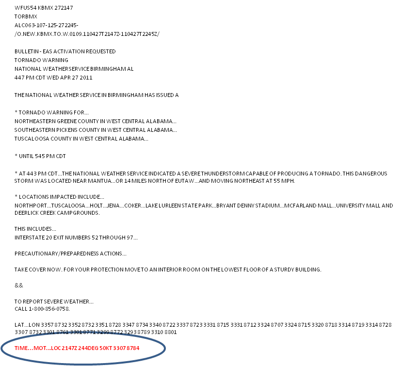
What about the placement of the point or line? Where should these go? Let’s just look at the point placement, the “Drag Me To Storm” position.
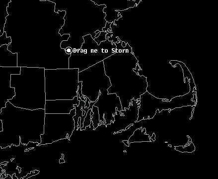
This point is used to represent the “storm”. But does this get placed at the centroid of the storm (option 1)? Or is it placed on the leading edge of the storm along the centroid motion vector (option 2)? Or the most forward portion of the echo (option 3)? Or elsewhere? This point is used to project the future location of the threat at the end of the warning, and also to compute the “pathcast” information. But if the point doesn’t actually represent the full spatial extent of the threat, wouldn’t the resulting polygons and pathcasts be incorrect? For example, if using the centroid of the storm, the severe weather might commence before reaching the centroid of the storm, and the polygons and pathcasts would be lag in time.
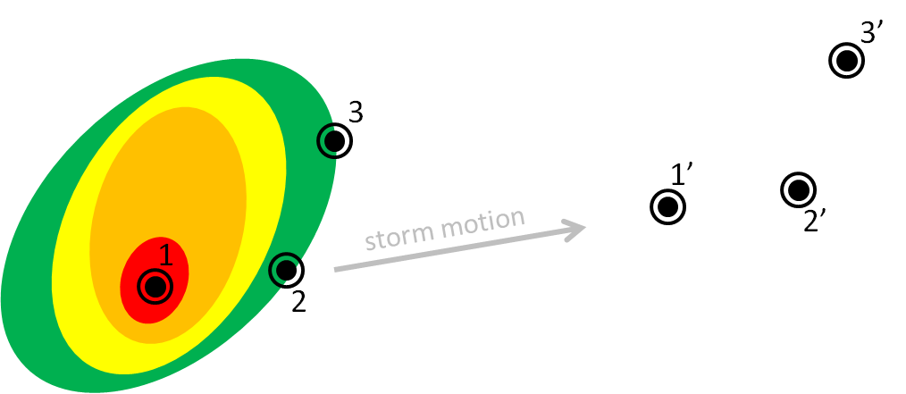
So let’s say for example we track using the storm centroid. Without editing the default polygon, you can see that a portion of the storm threat might be missed using the default box sizes. One could manually edit the polygon, but this would be done entirely qualitatively. How could this be done quantitatively?
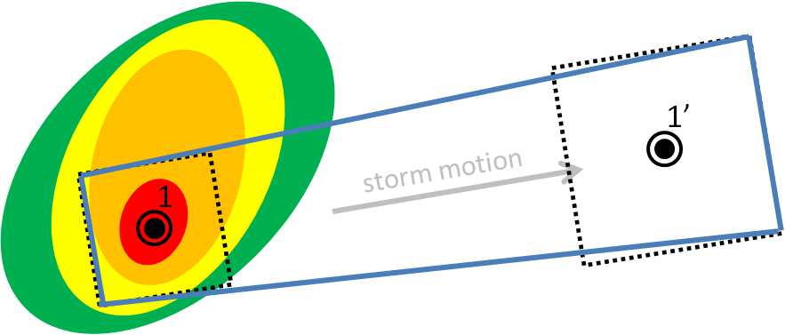
In either case, the storm hazard isn’t a point, but it is a two-dimensional area. In a way, WarnGen provides a 2D threat area, but it is a perfect square 20 km on each side. No storm actually has those dimensions. It therefore makes more sense that we should be defining 2D threat areas, and projecting 2D threat areas at future positions, like so (assuming the orange contour represents the spatial extent of the severe weather in this storm):
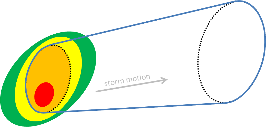
In addition, the future threat area defaults to a set expansion rate (exactly 150% its original size), and there is no direct way for the forecaster to quantify how much the threat area will expand, or how the projected area should be modulated to account for motion uncertainty or storm evolution.
We’ll show you one method in which we can address these shortcomings of WarnGen next, a proposed method for creating the short-fused convective hazard grids that does a better job at quantifying and directly coupling current and projected threat areas, motion, and motion uncertainty. In addition, this new warning generation methodology can provide intermediate threat area locations within the entire swath of the warning, plus one other major benefit: Threats-In-Motion (TIM), to be described very soon in this blog.
This is the first step in a proposed new hazard information delivery methodology that we feel will naturally dovetail toward the future “Warn-On-Forecast” paradigm of using numerical ensemble guidance to predict storm evolution beyond simple detection and extrapolation of threats.
Greg Stumpf, CIMMS and NWS/MDL
Let’s address the second and third shortcomings of WarnGen, (b) There is no way to adjust the motion vector for uncertainty. This must be done as a guess by manually editing the polygon vertices; (c) There is no way to change the default choice for the initial or projected threat areas. The same parameters (10km, 15km) are always used, and a square area is always the default.
In WarnGen, the forecaster can only choose one motion vector, and is limited to only one expression of uncertainty in the motion – the increase in the size of the warning area to a square with an area 225% larger than the initial threat area square. What if the forecaster determines that the storm is moving into an environment that is supportive of an evolution to a supercell, and the storm slows its forward speed and turns to the right (increasing azimuth in the motion vector)? The practice that is typically being suggested is to edit the vertices of the polygon to include more area to the right of the motion vector:
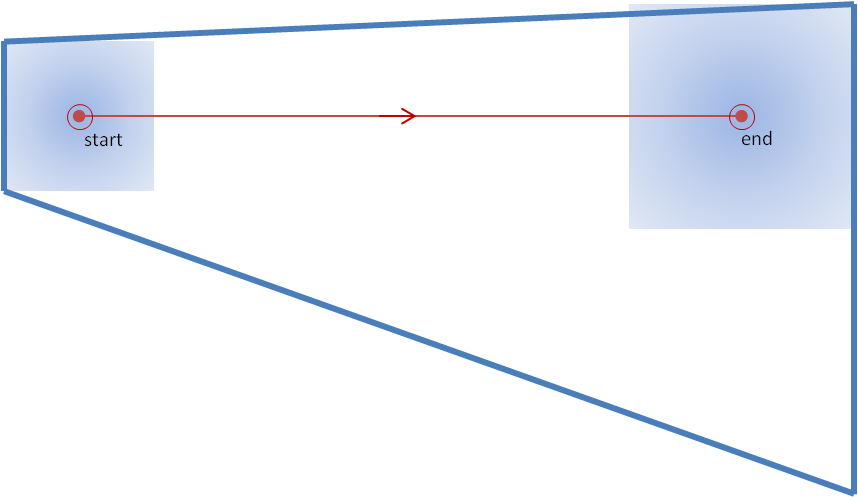
But how does the forecaster determine how far to the right to re-position the vertex? It’s another guess! Just click the vertex, drag it until it “looks about right”.
What would be the more robust way to determine how far to stretch the polygon? By being able to input information about the motion uncertainty in the form of a possible variance in the motion vector. For example, if the forecaster thinks a storm has a chance to slow and move to the right of the current motion vector based on the “30R75” technique (30 degrees to the right, 75% of the speed), then that information could be input to determine the possible locations of the threat area at the extrapolated final position of the threat. Here, I’ll only show the default threat position, and the 30R75 threat position:
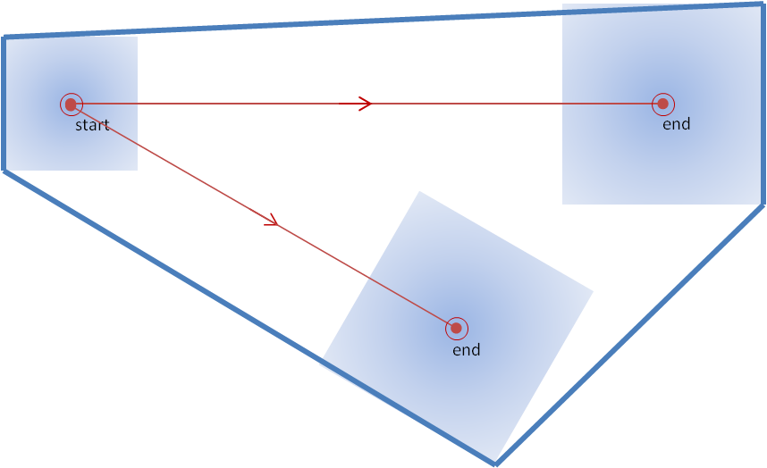
This looks similar to the “skewed coffin technique” offered by Nietfeld, but in this case, the position of the second solution is based on actual motion uncertainty numbers input by the forecaster, rather than a guess.
This is still not the ideal solution for determining the swath shape based on storm motion vector uncertainties. We’ll get to that soon.
Greg Stumpf, CIMMS and NWS/MDL
In the next set of blog entries, you are going to hear a lot more opinion and ideas of where some of us in the National Weather Center (NWC) community in Norman think we can begin to exploit technology to improve the way the NWS delivers hazardous convective weather information to its customers. It should be noted that these ideas are still in the process of being vetted across many disciplines: meteorology, technology, social science, ergonomics, etc. It has been a challenging process, namely because the resources to carry this out have been hard to come by. But we have been able to exhibit some of these ideas to NWS forecasters via the NOAA Hazardous Weather Testbed (HWT) and a social science stakeholder workshop and gained their valuable feedback. Our overarching goal is to improve the digital communication of hazard information to provide the best decision support services to the entire spectrum of users that the government serves.
So let’s continue by examining some of the shortcomings of the WarnGen function in AWIPS. Bear in mind that these comments are not meant to disparage the excellent work that the developers have done, but to highlight how we can evolve into an improved and more robust system to deliver hazardous weather information. Many of our concepts have been introduced at the first two Integration Hazard Information Systems (IHIS) workshops and are being considered by the GSD developers as the framework for the IHIS software is developed.
As you recall from earlier blog posts, WarnGen creates its default polygons thus:
1. Forecaster drags a point or line to a location on the storm at the current time
2. Forecaster steps the radar data back in time and drags the point or line to a location on the storm at some past time
3. The distance and bearing between the two points/lines, along with the time difference of the two radar frames, is used to determine a motion vector for that storm.
4. The forecaster selects a warning duration.
5. The point/line is extrapolated to its calculated position based on the motion vector and warning duration.
6. Around the initial point/line is drawn a 10 km buffer to represent the current threat area (20 km back side for point warnings).
7. Around the extrapolated point/line is drawn a 15 km buffer to represent the forecast threat area (30 km front side for point warnings).
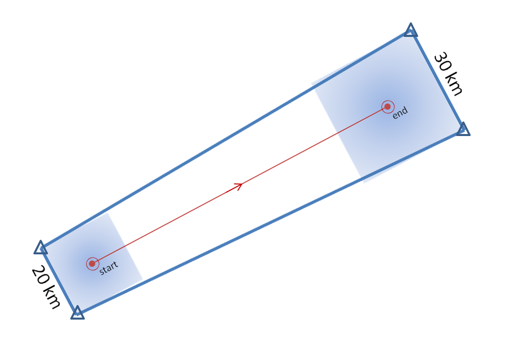
8. The back corners of the current threat area are connected to the forward corners of the forecast threat area to create default polygon. See here again, for a point-based polygon:
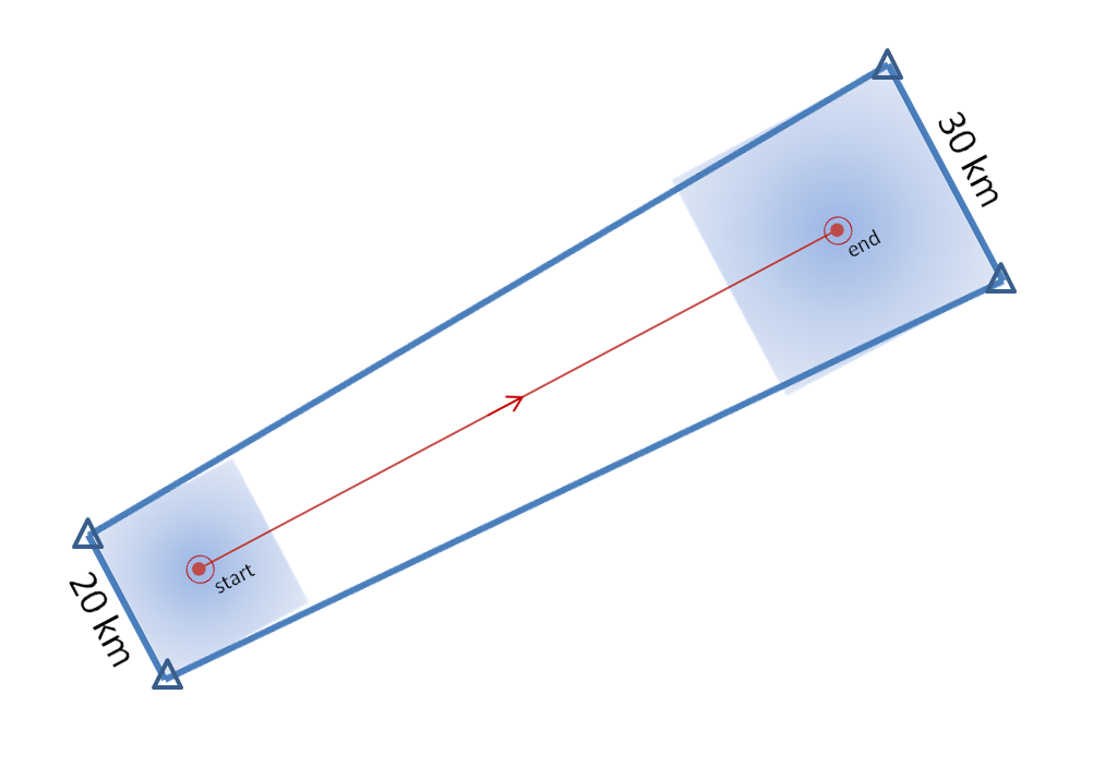
9. This polygon can then be edited by adding, deleting, or modifying any of the vertices (the triangles in the above figure).
10. The warning polygon is transmitted with accompanying text.
Here’s a list of some of the shortcomings to this process:
a. If any of the vertices of the polygon are changed, the polygon is no longer coupled to the motion vector, duration, and the initial and projected threat location.
b. There is no direct way to quantify motion uncertainty. This must be done as a guess by manually editing the polygon vertices.
c. There is no way to change the default choice for the initial or projected threat areas. The same parameters (10km, 15km) are always used.
d. Information about the intermediate threat area locations is not part of the warning. The polygon represents only the swath of the threat swept out through the duration of the warning.
e. If the storm changes its predicted evolution (motion vector, grows, shrinks, splits, etc), there is no way to adjust the polygon swaths without (in most cases) having to issue another polygon to account for the change.
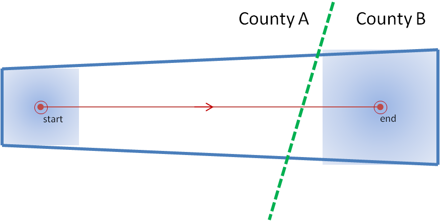
Let me first address limitation (a). Let’s take a look at a situation that we’ve observed a number of times with warnings, and is actually taught as a “best practice”. A warning polygon is issued that covers two counties. The downstream end of the polygon extends not too far into the next county. The warning forecaster does not have enough confidence that the storm will remain severe into the end of that county, so the forecaster “clicks off that county” (this can be done within Warngen – counties can be removed or added at the click of a mouse.) The warning is then transmitted. See anything wrong here?
Let’s look at this in pictures. Here’s the original warning polygon, with the county borders included. Let’s assume that this warning is in effect for 60 minutes:
And here is the new warning polygon after County B has been “clicked off”:
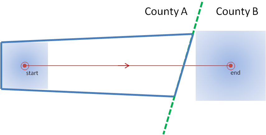
I’ve left the background extrapolated threat point and area on the second figure. Note that the warning polygon was edited and then transmitted. An important step was omitted! Assuming that storm moves exactly as extrapolated, where will that storm be in 60 minutes? Located at the end point. When will that warning polygon expire? When the storm is located at the end point. Is the storm inside the polygon? No! The storm exited the polygon well before the polygon expired. If the forecaster was relying on an alerting application (such as SevereClear) to announce that the warning was nearing expiration, the forecaster may get the alert well after the storm as already exited the polygon, and the storm becomes unwarned! The storm escaped its cage and is on the loose!
Some warning forecasters will account for this issue before transmitting the polygon by reducing the duration of the warning. But how is the new duration chosen? How does the forecaster know exactly at what time the storm will be at the end of the shortened warning? They really don’t, and they have take a guess.
How should the warning be adjusted for uncertainty of duration? Not by editing the polygon, which should represent the accumulated swath of all the extrapolated positions of the threat area from the current time, through all intermediate positions, to the final position. Instead, it should be done by adjusting the duration of the warning, thus affecting the final extrapolated position of the threat. Here’s the same warning with a 40 minute duration (note that even though I slightly clipped the county, I don’t advocate this in the purest sense):
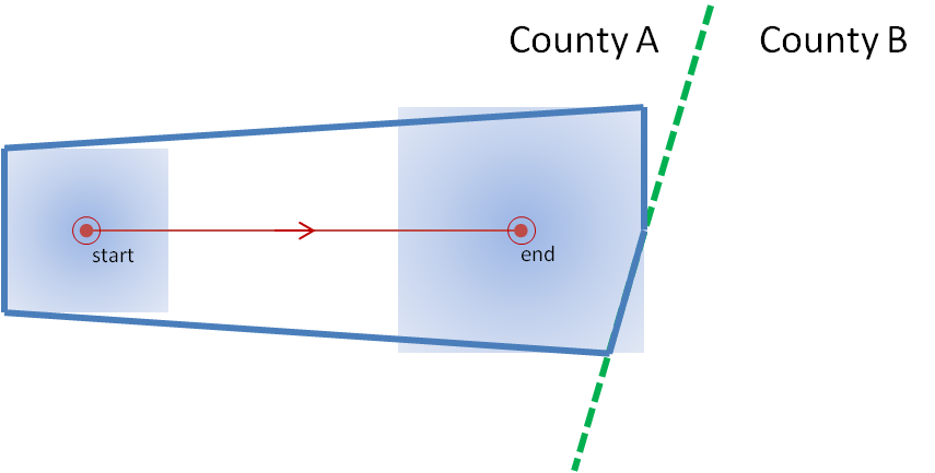
Yes, this can all be done carefully using WarnGen, but we have a better idea how the warnings swaths should be created. This new idea will also address the other shortcomings, which I will describe next.
Greg Stumpf, CIMMS and NWS/MDL
In the previous post, I examined the affects of warnings with more area on a single isolated long-tracked tornadic storm. Now let’s look at a typical event that can comprise multiple tornadoes from independent mesocyclonic circulations, namely tornadoes along the leading edge of a Quasi-Linear Convective System (QCLS). These are typically more challenging than supercell tornadoes to warn for because their existence, timing, and location can be more uncertain. An example QLCS system with 5 vortices along the leading edge of the gust front is depicted here:
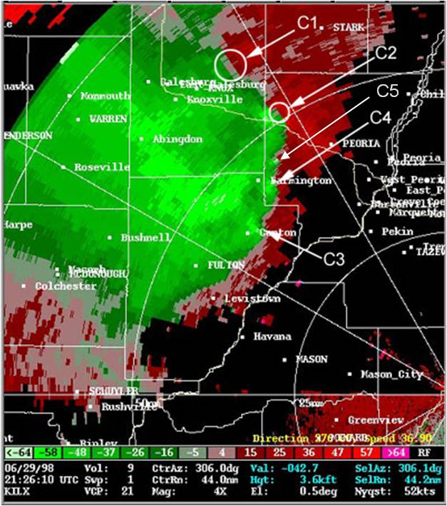
How are these situations warned for today? Well, the strategies vary from WFO to WFO and from warning forecaster to warning forecaster. In some instances, the large uncertainty of the event and sometimes high workload encourage forecasters to “cast a wide net” over the entire leading edge of the QLCS system with a single large and long Tornado Warning in hopes of not missing any tornado that might occur. However, this may result and large areas falsely warned for considerable amounts of time. But if there are no tornadoes, it’s only one false alarm. One of the pitfalls of our current warning verification system!
In other instances, forecasters might be more conservative and wait until a signature becomes apparent, and issue a smaller more-precise Tornado Warning for just that particular circulation. However, in these instances, sometimes the warnings come late, resulting in either small lead times, or negative lead times with some or all of the portions of the tornadoes being missed.
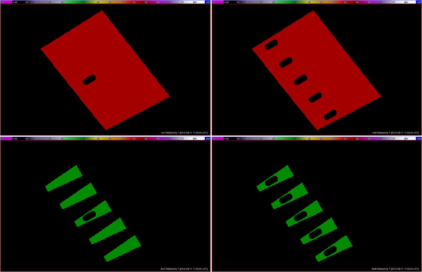
Let’s look at how both warning methodologies stack up when verified geospatially for a simulated QLCS event. For the simulation, I created 5 parallel mesocyclone tracks that were 40 km apart, each starting and ending at the same time with a 60 minute duration and moving with the same motion vector (about 25 m/s from the southwest to the northeast). As with the Tuscaloosa case, I used the mesocyclone centroid locations to determine the storm motion vector and position of the warning polygons, simulating a storm motion forecast with perfect skill using careful radar analysis.
I ran two warning methodologies. In each case, the warnings expire after their intended duration and are never modified using the Severe Weather Statement (SVS) reduction method during their durations. The warnings start at the same time in each scenario.
1warn: Issue one large warning using the default AWIPS WarnGen “line warning” polygon with an expiration time of 60 minutes. To create the warning, a line is drawn from the centroid of the first mesocyclone to the centroid of the fifth mesocyclone at the beginning time of the warning. This line is projected ahead 60 minutes using the storm motion vector. A 10 km buffer is drawn surrounding the beginning line and a 15 km buffer is drawn around the ending line. These are the same parameters used to create the default AWIPS WarnGen polygons for line warnings. The far corners of each buffer are connected to create a four-sided polygon. This is the “cast the wide net” scenario.
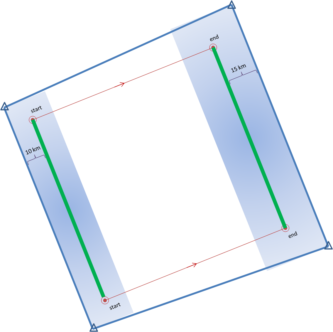
5warn: Issue five small warnings centered on each of the five individual mesocyclones. The warning durations are set for 30 minutes (half the duration). The warning polygon sizes are based on a 5 km buffer (10 km back edge) around the starting point of each warning, and a 10 km buffer (20 km front edge) around the projected ending point of each warning. Note that these are smaller than the default buffer sizes, and are chosen so to simulate a more precise warning for what are typically short-lived tornadoes. This is the “high precision” scenario.
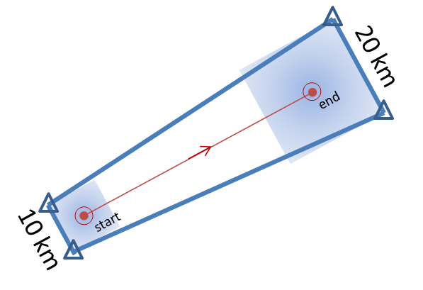
I then vary the outcome, the verification of the tornado events, in two ways:
1torn: Only one tornado: The middle (third) mesocyclone produces a tornado 10 minutes after the warnings were issued, lasting exactly 10 minutes. The other four mesocyclones are non-tornadic.
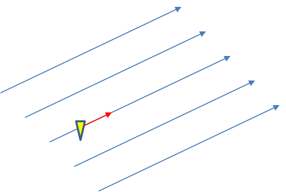
5torn: Five tornadoes: All five mesocyclones produce a tornado 10 minutes after the warnings were issued, each lasting exactly 10 minutes.
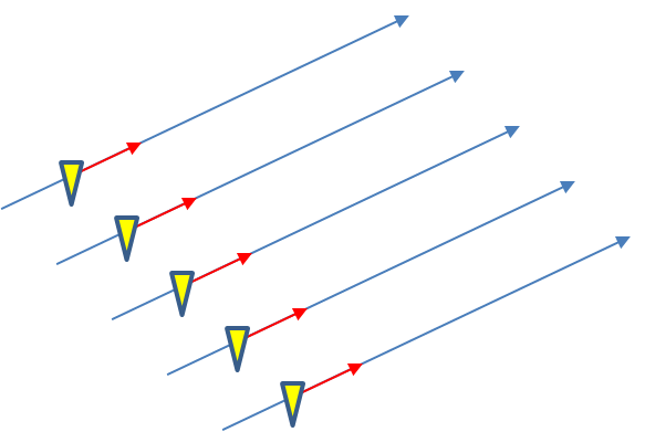
The four scenarios are illustrated in the figure below. In each case, the dark regions inside the polygons represents the area swept out by the simulated tornadoes with a 5 km splat radius added.
Let’s first consider the traditional warning verification stats for these four scenarios:
1warn-1torn: POD 1.0, FAR 0.0, CSI 1.0
5warn-1torn: POD 1.0, FAR 0.8, CSI 0.2
1warn-5torn: POD 1.0, FAR 0.0, CSI 1.0
5warn-5torn: POD 1.0, FAR 0.0, CSI 1.0
All but one of the scenarios results in prefect warning verification. Scenario 5warn-1torn, 5 precise warnings and only one tornado, results in 4 “false alarms”.
Now, how do these scores compare to using geospatial warning verification, where only one 2×2 table is used, and large false alarm area and times are considered poor performance? Using the “grid point” verification method:
1warn-1torn: POD 1.0000, FAR 0.9993, CSI 0.0007
5warn-1torn: POD 1.0000, FAR 0.9942, CSI 0.0058
1warn-5torn: POD 1.0000, FAR 0.9966, CSI 0.0034
5warn-5torn: POD 1.0000, FAR 0.9709, CSI 0.0291
And using the “truth event” verification method:
1warn-1torn: POD 1.0000, FAR 0.9894, CSI 0.0106
5warn-1torn: POD 1.0000, FAR 0.9544, CSI 0.0456
1warn-5torn: POD 1.0000, FAR 0.9471, CSI 0.0529
5warn-5torn: POD 1.0000, FAR 0.7726, CSI 0.2274
Using each of these verification methods, the scenarios in which 5 separate precision warnings are issued have lower FARs and higher CSIs versus the large long-duration warning decisions for both the 1-tornado event and the 5-tornado events respectively. In addition, there is the obvious difference in the scores when comparing the aggregate false alarm times for each scenario:
1warn-1torn: FAT 1,101,120 km2-sec
5warn-1torn: FAT 123,660 km2-sec
1warn-5torn: FAT 1,054,020 km2-sec
5warn-5torn: FAT 100,110 km2-sec
The 5 precision warnings result in total false alarm times that are about 1/10th of the large long-duration warnings. So even given the case that 5 precision warnings are issued and only one tornado results, the time and area under false alarm is greatly reduced.
From a services standpoint, in the 5 precision warning case, there will be 5 separate alerts, 4 resulting in no tornado. However, for the large warning scenario, there may only be “one alert”, but 10 times the area and time receiving the alert result in no tornado. How do we deal with the issue that there will be more false alerts for the precision warning method? We change the way we alert! More later…
ADDENDUM: Jim LaDue of the NWS Warning Decision Training Branch (WDTB) wrote an excellent position paper describing why we should not adopt a practice to avoid issuing Tornado Warnings (and instead use Severe Thunderstorm Warnings) for the perceived notion that QLCS tornadoes are weak (EF0 and EF1). Makes for excellent reading!
Greg Stumpf, CIMMS and NWS/MDL
Geospatial warning verification addresses both of the pitfalls explained in earlier blog entries by consolidating the verification measures into one 2×2 contingency table. The verified hazards can be treated as two-dimensional areas, of which they are – storm hazards do not affect just points or lines! We can include the correct null forecasts in the measures. This method provides a more robust way to determine location-specific lead times as well as new metrics known as departure time and false time. In addition, the method will reward spatial and temporal precision in warnings and penalize “casting a wider net” by measuring false alarm areas and false alarm times, which may contribute to a high false alarm perception by the public.
How might we measure the effect of the last issue addressed? Let’s take our Tuscaloosa example and see what the effect of varying the warning size and duration has on our verification numbers. I will only present a few test cases here, because I want to eventually explore this further with a different storm case that isn’t comprised of a single long-tracked isolated storm.
I developed a method which will take my truthed mesocyclone centroid locations and use them to compute the storm motion vector as specific warning decision points along the storm track. Starting from the initial warning decision point from the BMX WFO on the TCL storm (2038 UTC 27 April 2011), I created warning polygons using the default AWIPS WarnGen polygon shape parameters. Namely, the current threat point is projected to its final position using the motion vector and a prescribed warning duration. A 10 km buffer is drawn around the starting threat point resulting in the back edge of the warning being 20km. A 15 km buffer is drawn around the ending threat point resulting in the back edge of the warning being 30km. The far corners of each box are then connected to create the trapezoid shape of the default warning polygon.
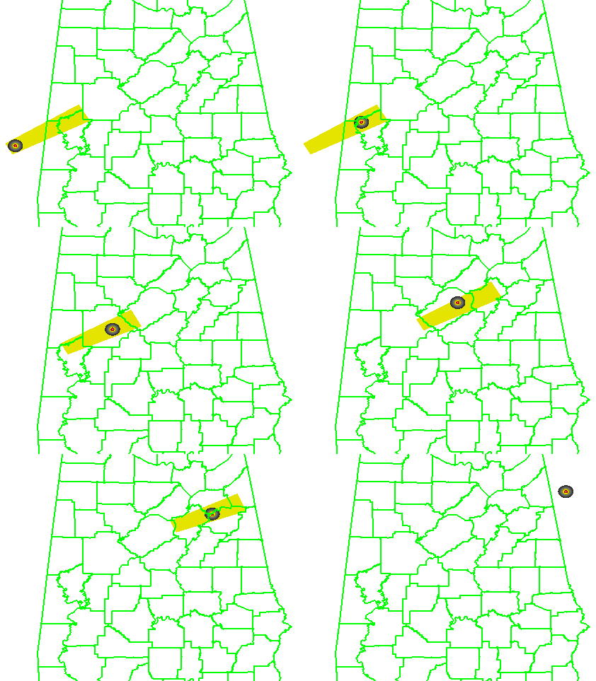
I used a 60-minute warning duration since the NWS warnings were also about 60 minutes in duration for the TCL storm. I have a re-warning interval of 60 minutes, so that a new warning polygon is issued as the hazard location is nearing the downstream end of the current warning polygon. Because of the buffer around the projected ending point of the threat, each successive warning will have some overlap with the previous warning, which is considered a best warning practice. None of the warnings will be edited for shape based on any county border, because we want to test the effect of warning size and duration without any other factors influencing the warning area. A loop of the warning polygons with the mesocyclone path overlaid:
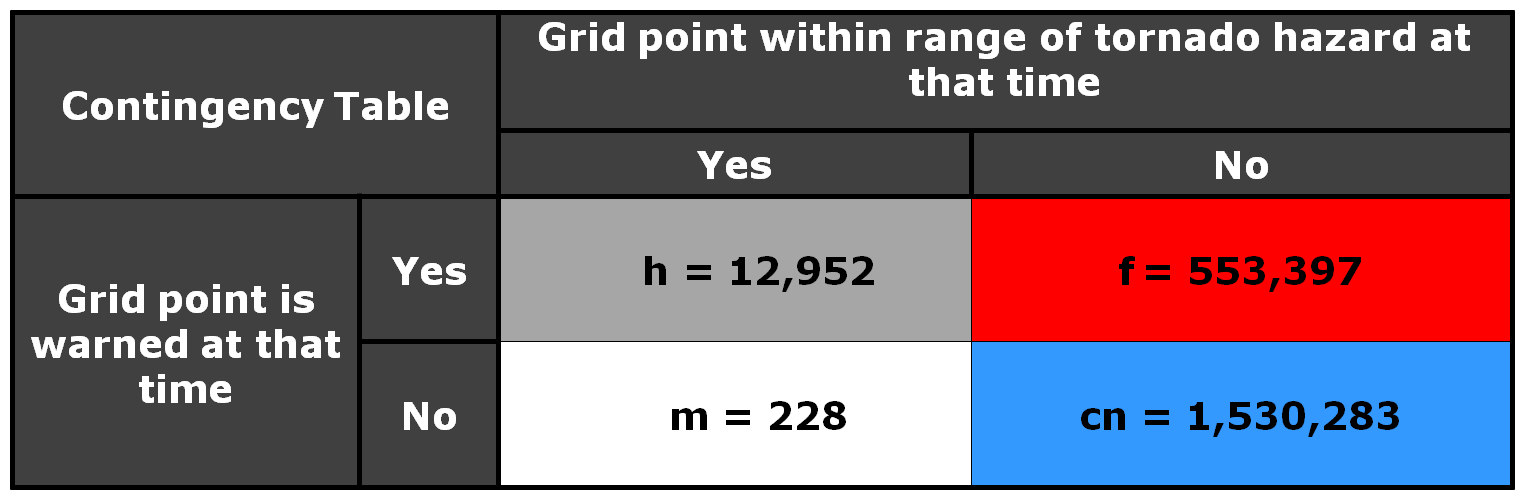
Here is the 2×2 table using a 5 km radius of influence (“splat”) around the one-minute tornado observations, I am not applying the Cressman distance weighting to the truth splats, and I’m using the composite reflectivity filtering for the correct nulls:
And the grid point method scores are:
POD = 0.9827
FAR = 0.9771
CSI = 0.0229
The FAR and CSI are slightly better than the NWS warnings. However, I’m not trying to compare this method to the actual warnings, but rather as a start to determine the effect of larger and longer warning polygons. So, let’s try that now. Instead of using starting and ending box sizes of 20 and 30 km respectively for our default WarnGen polygon, let’s cast a wider net and quadruple that to 80 and 120 km. The polygon loop would look like this:
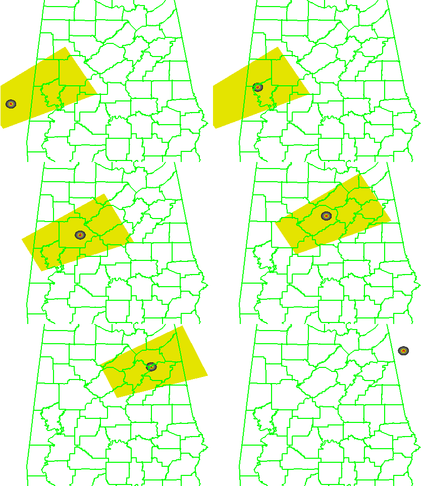
And the 2×2 table and scores like this:
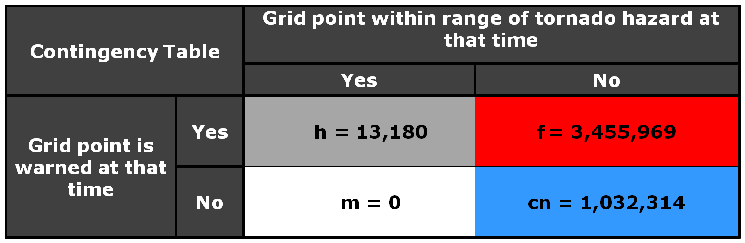
POD =1.0000
FAR = 0.9962
CSI =0.0038
What was the effect of the larger longer polygons? Well first, there were no missed grid points, and the POD = 1. But the number of false alarm grid points increased by a factor of about 7, and thus the FAR went up and the CSI went down. Recall that the number of false alarm grid points represents the number of 1 km2 grid points accumulated for each minute of data, so the false alarm area and time are much larger, even though these warnings verified perfectly.
So let’s take this in the opposite direction and make our warning polygons smaller. We’ll use starting and ending box sizes of 6 and 10 km respectively. The loop:
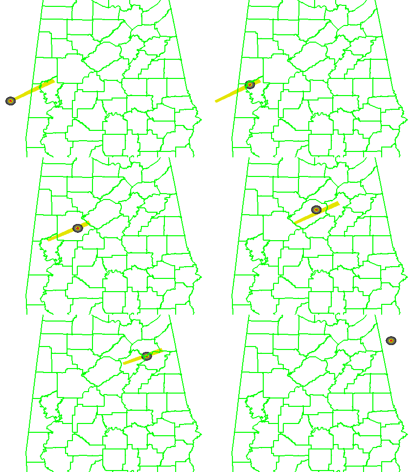
and the numbers:
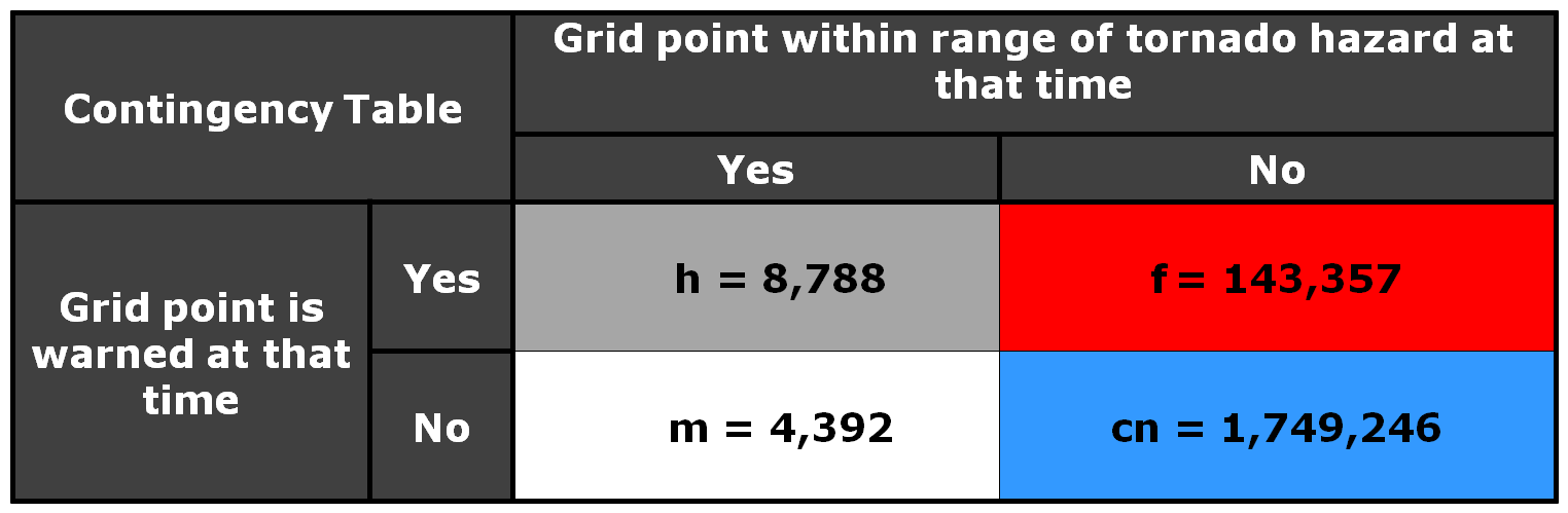
POD = 0.6668
FAR = 0.9422
CSI =0.0561
We’ve significantly reduced the false alarm area, but we also negatively affected the POD. About 1/3 of the tornado grid points were missed because the warnings were too small.
Now, let’s run the “Truth Event” statistics on all three scenarios:
3 km: pod 0.6390, far 0.3041, csi 0.4995, hss 0.6563, lt 32.8, dt 27.4, ft 61.8
10 km: pod 0.9968, far 0.6780, csi 0.3217, hss 0.4619, lt 39.0, dt 32.1, ft 71.3
40 km: pod 1.0000, far 0.9164, csi 0.0836, hss 0.1015, lt 73.2, dt 46.7, ft 114.6
The 3 km warnings have the best CSI and HSS. This appears that the geospatial verification scheme is rewarding more precise polygons. But there is a problem…there is also a pretty low POD, which means that portions of the tornadoes are not being warned. That’s not good, and reflective of the Doswell “asymmetric penalty function” where forecasters are harmed more by missed tornadoes than false alarms. Why is this so? Because our warnings are being issued for 60 minute durations and 60-minute re-warning intervals. That means for these narrow warnings, if the storm motion deviates after the warning is issued, then there is no chance to re-adjust the warning to account for the storm motion changes. Hence, a larger warning would capture these changes.
One might wonder – how can we balance precision and high POD? I will treat this issue in a later blog, but for now, the next entry will continue to look at the issues of casting a wider net as it pertains to a very hot topic right now – how to warn for Quasi-Linear Convective System (QLCS) tornadoes.
Greg Stumpf, CIMMS and NWS/MDL

We can dissect the stats a little more. First, let’s look at the overall distribution of LEAD TIME (LT), DEPARTURE TIME (DT), and FALSE TIME (FT) for all truth events to get an idea about the range of values. The following histograms depict the distribution of values for each grid point. These graphs show a lot more information than the average values for each presented in the last blog post.
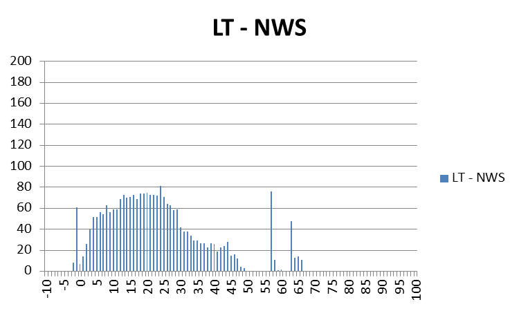
For LEAD TIME (LT), you can see that for some of the grid points, there were some negative lead times, and a fair number of grid points with lead times below 10 minutes. Also note the few grid values above 55 minutes. These were caused by the start of the two tornadoes forming at the very far ranges of the warnings covering their storms. Looking at the lead times for just the starting time of those two tornadoes, the numbers end up being fantastic: 65 minutes and 57 minutes respectively, according to the NWS Verification statistics. But as we are showing here, it is important to consider the lead time between warning issuance and tornado impact at each specific location along the path of the tornado, and for some of those, the numbers don’t reflect as good a level of success as those two numbers above. We will explore this further in just a second.
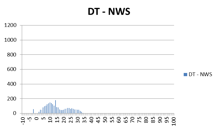
For DEPARTURE TIME (DT), we can see that warnings were cleared out anywhere from 0 minutes to as much as about 35 minutes after the threats had passed. Should warnings remain in effect for so long? The clearing of warning polygons via Severe Weather Statements (SVS) serves this purpose, but it is a manual process that does not have a standard protocol from WFO to WFO, and sometimes isn’t done when workload is too demanding. Also note a few data points in the negative area – these are warnings that were cleared too early – the threat was still affecting those locations. However, recall that our threat locations have a 5 km splat radius around them; these data points come from the very back end of some of these splats at the early stages of the first tornado.
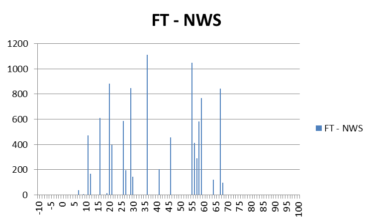
The FALSE TIME (FT) distribution looks much different than the other two, it is more “disjointed”. The main reason for this is because these values are based on the warnings and not the one-minute updating tornado threat locations, so there will be discontinuities associated with each change in the warning polygons, which comes about every 15 minutes as new warnings are issued or current warnings are reduced in size via SVS. But note that there are some locations that are falsely warned for over 60 minutes! This is even though the storm-based polygon warnings were technically not false alarms according to traditional NWS warning verification methods.
Because our data are geospatial, we have the luxury of looking at the geospatial distribution of the LT, DT, and FT values on a map! Let’s start with the LEAD TIME (LT) graphic:
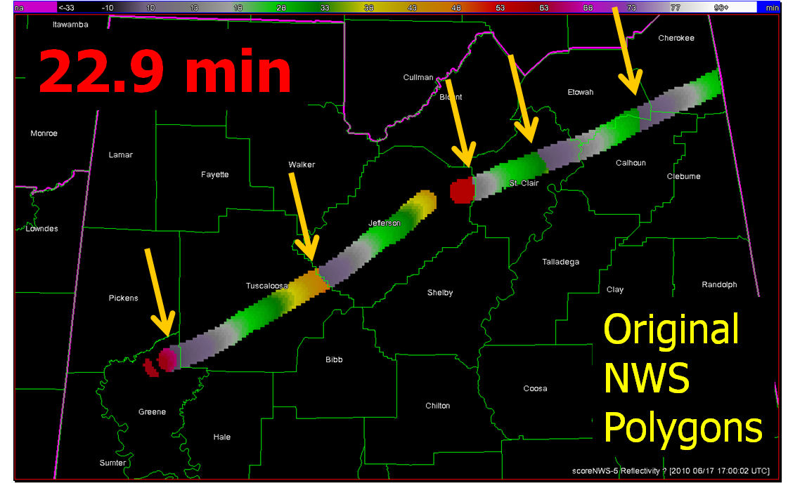
What you are seeing here are the LEAD TIME values at specific locations along the path of the two tornadoes, with the 5 km “splat” buffer added (no values are recorded outside the path of the threat). Pay particular attention to the five yellow arrows. We’ll zoom in on one of them:
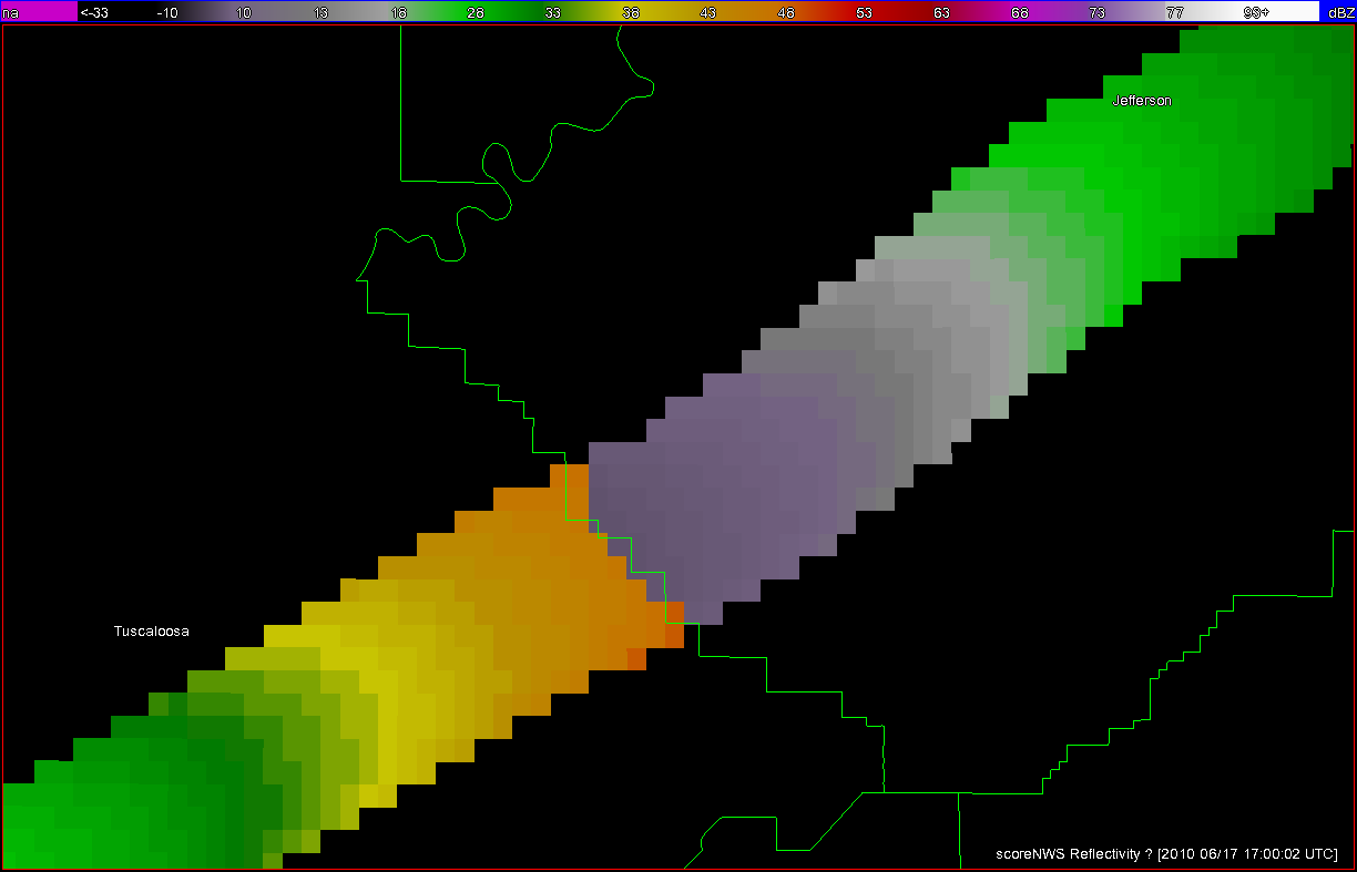
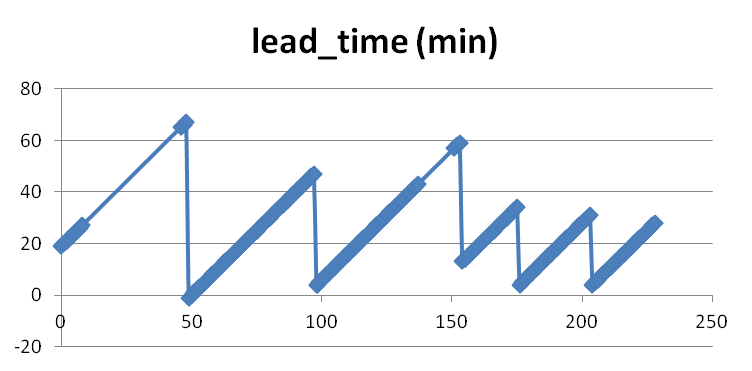
What we are seeing here is a discontinuity in LEAD TIME at this location of the tornado path. Values at the far end of Tuscaloosa County are 47 minutes, while at adjacent grid points downstream in Jefferson County, the lead times on the tornado path were only 3 minutes. These inequitablies are the result of warnings being issued one after the other, with the threats nearing the end of one warning polygon before the next downstream polygon is issued. This is evident in the NWS polygon warning loop I showed in a previous blog entry. There are five of these discontinuities in the path of both tornadoes from this storm. These five discontinuities represent the downstream end of the first five polygons that were issued by the NWS on this storm (the 6th polygon warning expired on the AL-GA state line, so the discontinuity is not seen because I didn’t include the grid points within Georgia). The same five discontinuities are also seen if we plot the one-minute tornado segment lead times available from the NWS Verification database:
The graphical DEPARTURE TIME map:
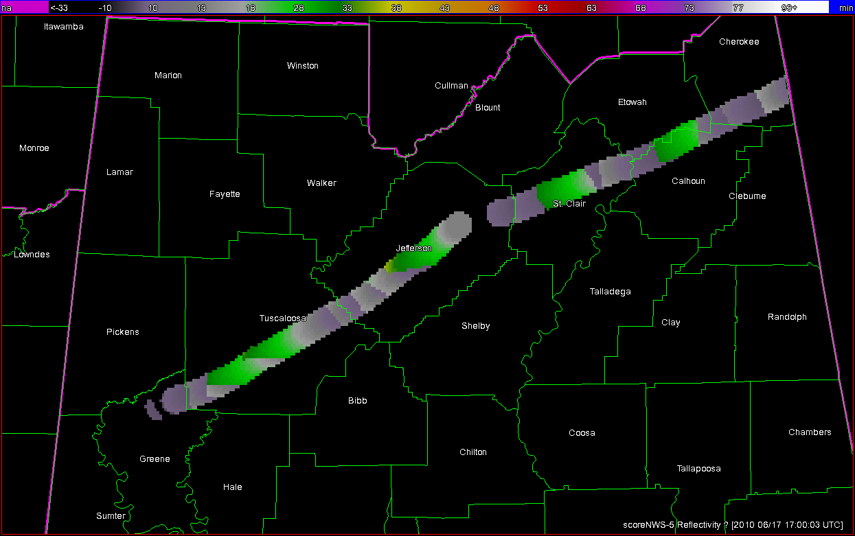
More discontinuities are seen here because in addition to the new warnings being issued, there were the numerous removals of the back ends of the polygons via the SVSs.
This final graphic depicts the FALSE TIME (FT) per grid locations. Values only exist where warning polygons were in effect outside the path of the tornado plus the 5km splat.
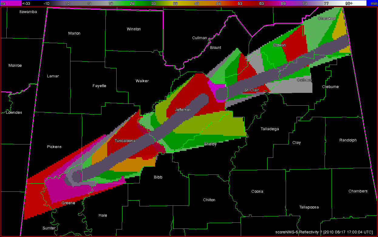
There is quite a bit of area that is falsely warned (assuming the 5 km buffer around the tornado), and many of these areas are warned for over 60 minutes. Note each warning polygon and subsequent SVS edit becomes evident on this graphic. Note too that for the second tornado the warning polygons are placed with the tornado path to the right of center (as viewed toward the storm motion direction), which indicates that the warning forecaster probably started using the Tornado Warnings to cover the entire severe threat (wind, hail) and not just the tornado threat.
Next up, a summary of the benefits of geospatial warning verification, and then an exercise illustrating the second pitfall of “casting the wider net”.
Greg Stumpf, CIMMS and NWS/MDL