EWP Blog – Page 46 – Spring Experiments & Beyond

Albuquerque HWT

Posted in NUCAPS, OCTANE Speed Sandwich, PHSnMWnABI, SPG2023 on June 7, 2023 by Kevin Thiel.

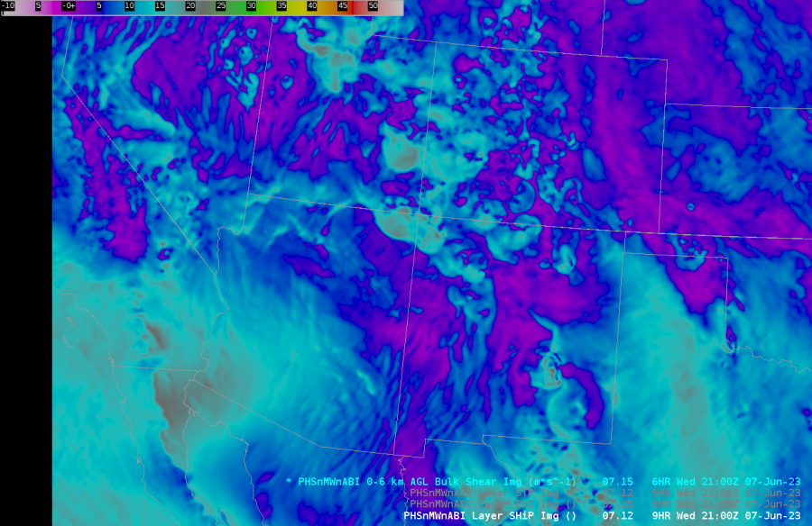
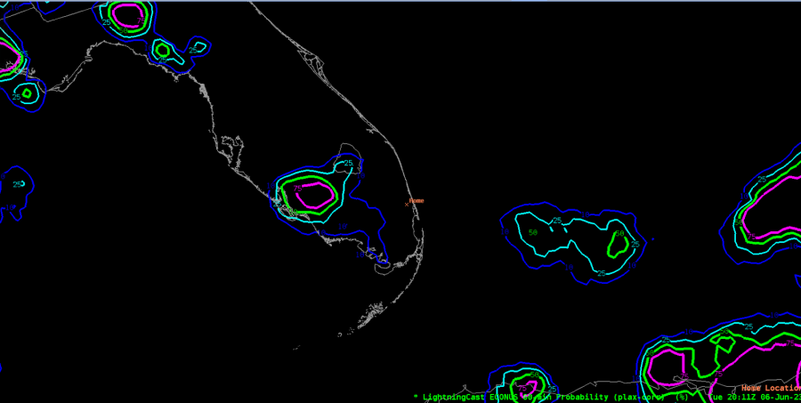
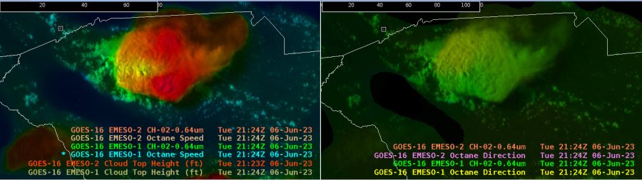
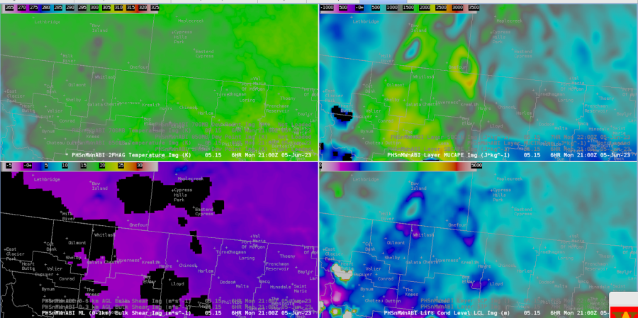
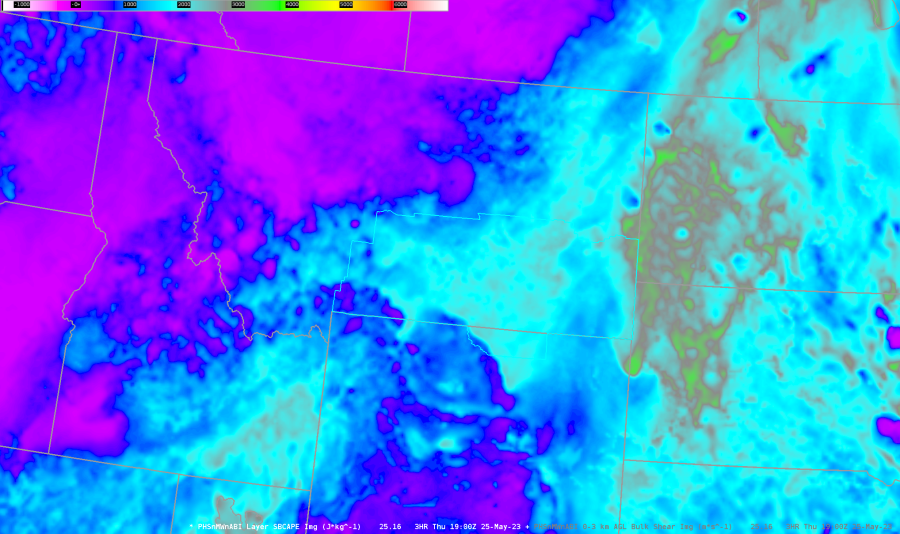
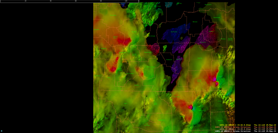
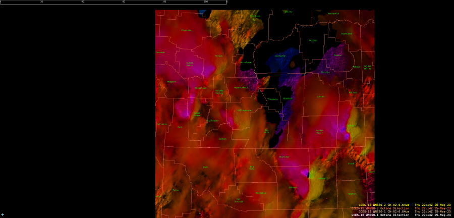
Storms are exhibiting some decent shearing aloft over NW New Mexico when comparing to NE New Mexico. Something I might not have noticed had I not had this product as I don’t always have time to go into the SPC mesoanalysis and check various levels of shear values. The 0-8km shear values are in the 40-50 kt range, in agreement with the range of values noted on the speed shear values of OCTANE. See below.

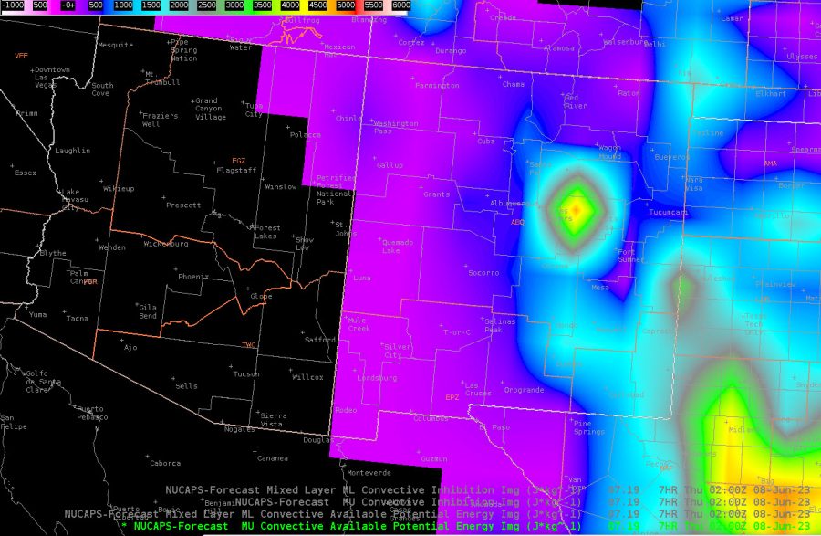
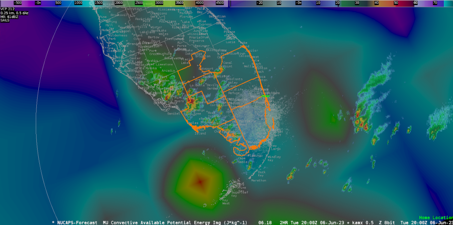
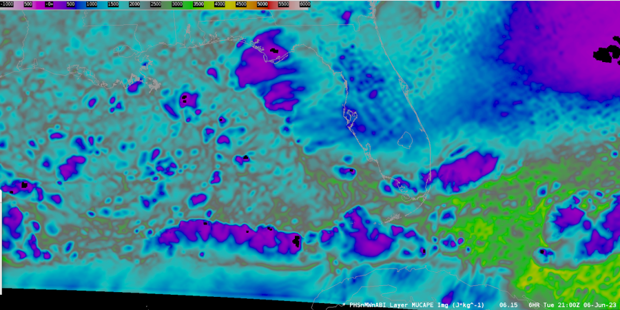
PHS really doing a nice job of pointing out peak areas of MUCAPE and where storms will likely develop. Decent scale and resolution results in some good quality comparisons with various other products. This is over the southern ABQ CWA.

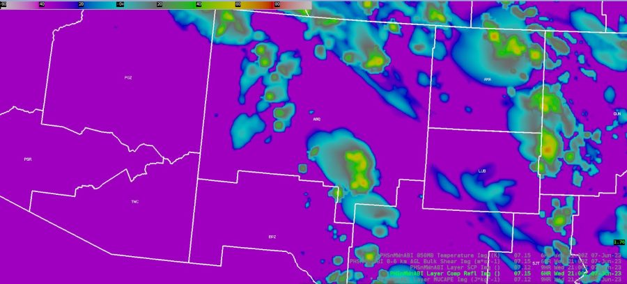
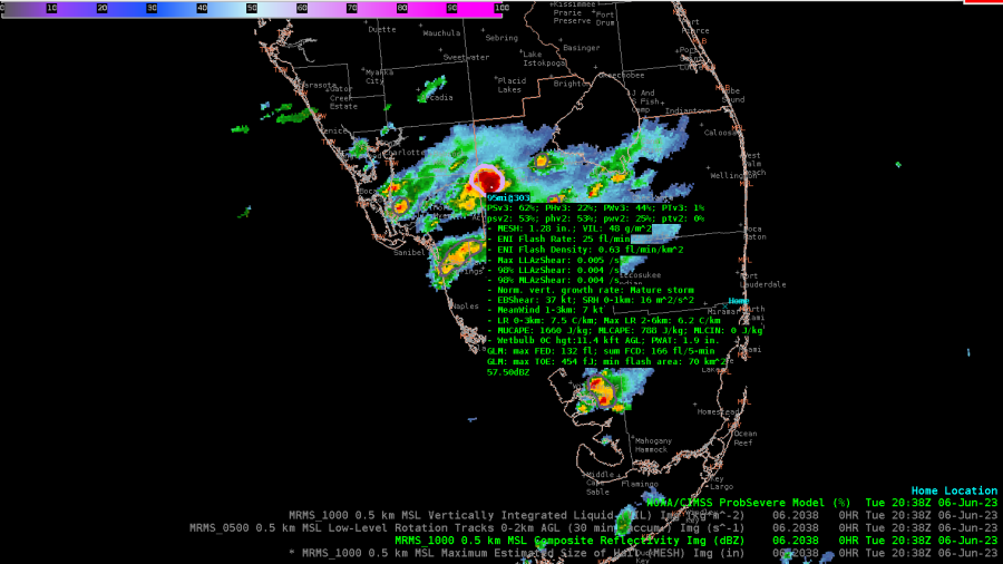
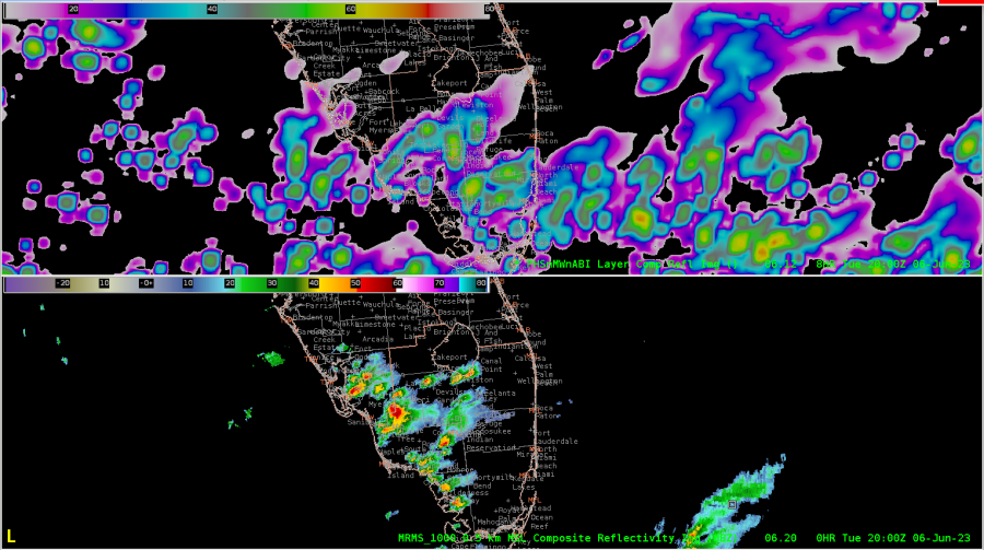
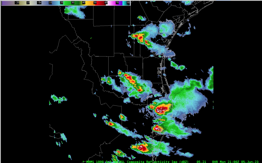
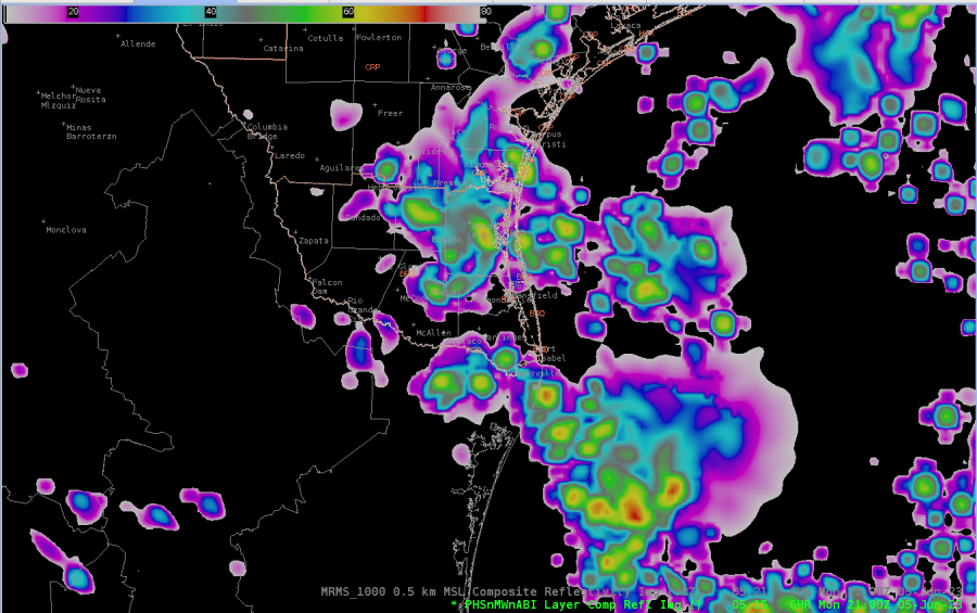
Forecast Layer Comp Refl 21Z

Forecast MUCAPE 21Z

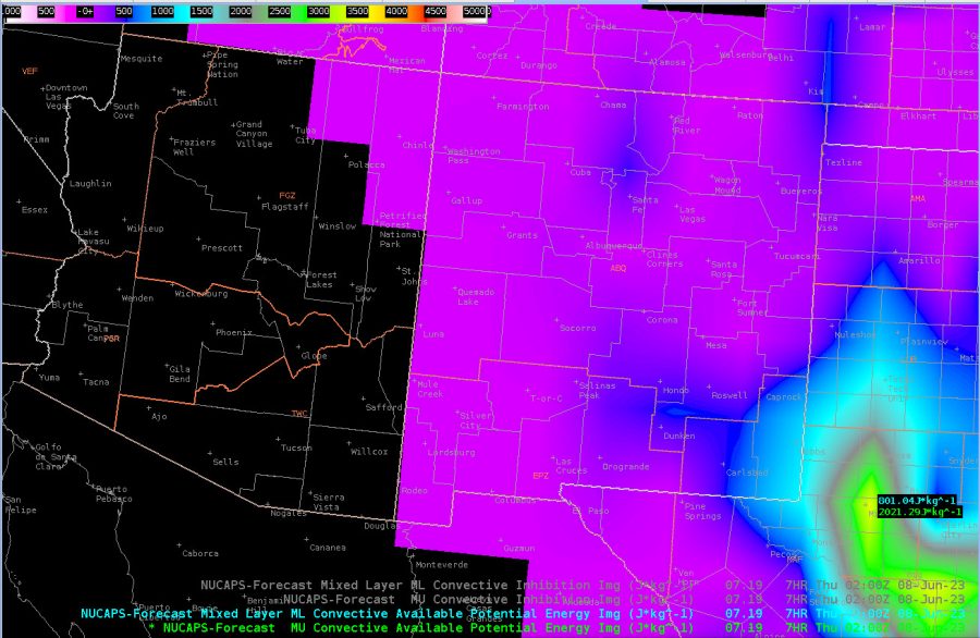
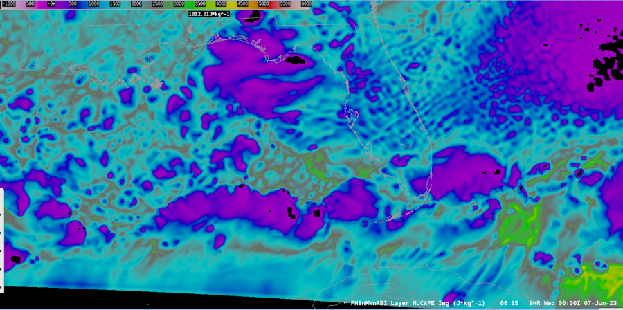
Forecast MUCAPE 23Z – Also, noting a sharp gradient in MUCAPE values as convection strengthens over east-central New Mexico late this afternoon into the early evening hours. We will have to see how this plays out.

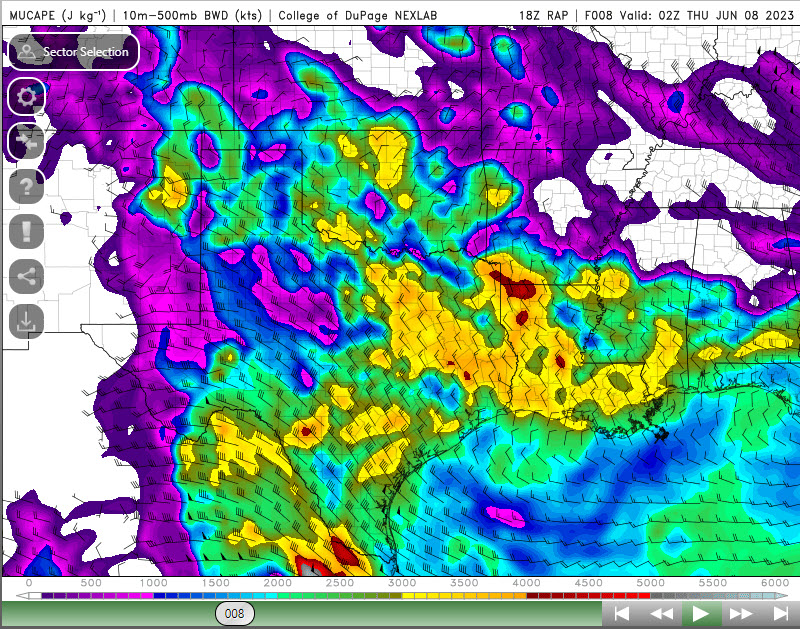
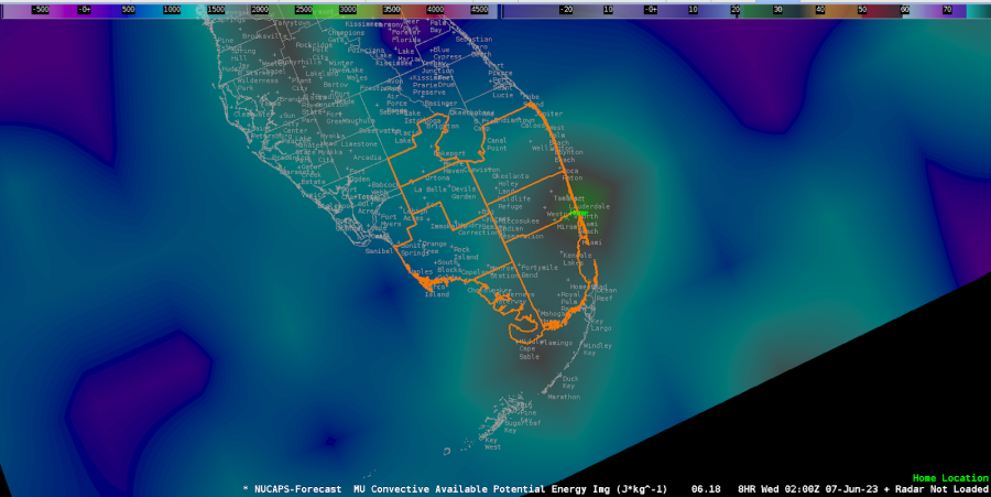
MUCAPE values seem a bit higher than they should be when compared with the MLCAPE values at the same times over New Mexico. I’m not exactly sure why the values are so high, but the forecast RAP values for the same time frame appear to be notably more displaced to the east and lower.

Example below from forecasted time 02Z.

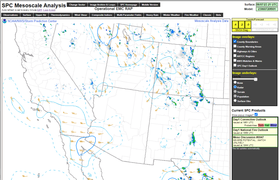
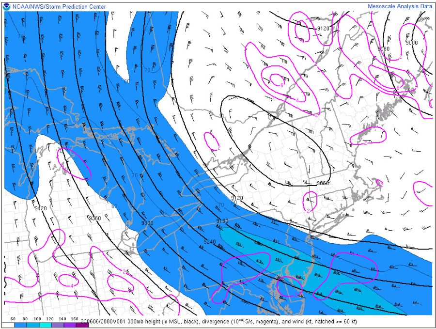
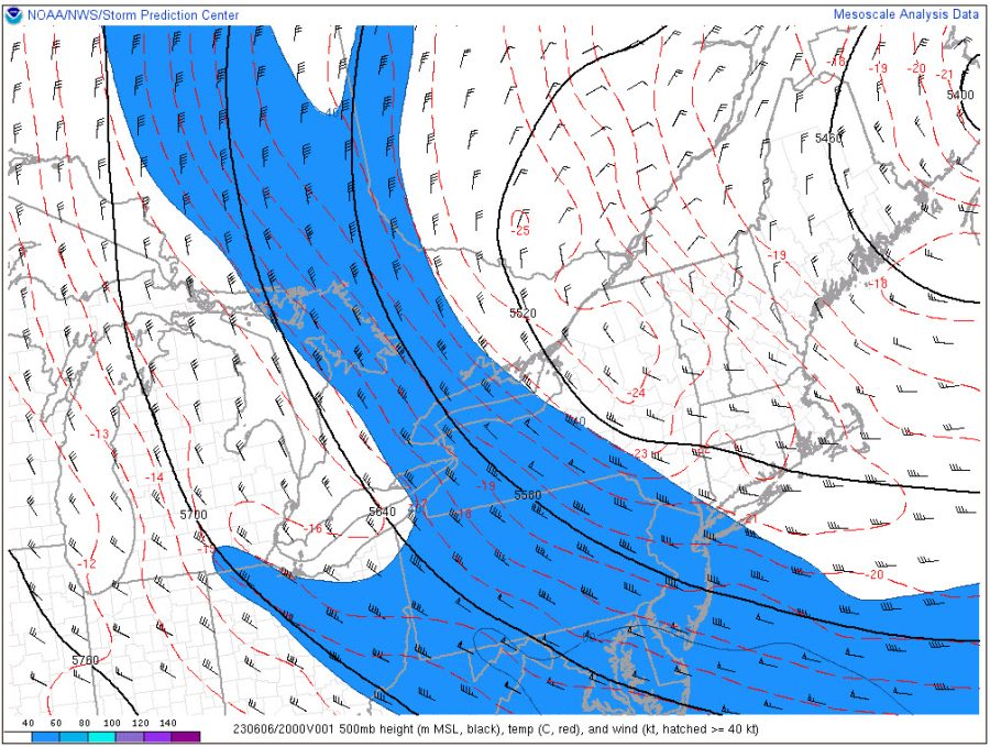
The 6 hour forecast at 21z of PHS 0-6 km Bulk Shear (first image) is compared against the 21z SPC Mesoanalysis (second image). Overall, the PHS forecast did quite well over New Mexico. There is generally little to no shear across the state except for near the Four Corners in the northwest and far southeastern New Mexico. The values are reasonable in these areas as well, around 16 m/s for PHS which fits in with the over 30 knot SPC values.These differences can be noted in the convection occurring as well (seen in the SPC image). Mainly isolated cellular over central NM, but showing more organization in the areas of higher shear.

-Satellite Steve and Burton Guster

Monitoring South FL Convection for the Miami Open

Posted in DSS, LightningCast, NUCAPS, OCTANE Speed Sandwich, PHSnMWnABI, ProbSevere, SPG2023 on June 6, 2023 by Kevin Thiel.

We’re closely monitoring for CI near the Miami Open Tennis Tournament (location noted by the Home marker). Thus far this afternoon, the deepest convection has been in the west, NE of Naples, where the Band 13 imagery shows high cloud tops with cool brightness temps (-66C), and Octane imagery shows a good divergent signal.

So far, LightningCast has focused on the convection in the western peninsula, with the maximum slowly translating inland and to the N along the inland-tracking sea breeze.

This is further confirmed by the lightning meteogram for the DSS site. Looks like they can keep playing tennis for a little bit longer!

Looking at the storm clusters back west, a NUCAPS sounding near that cell shows plenty of CAPE.

The NUCAPS-Forecast MUCAPE confirms the high CAPE invof the storms.

Let’s see what the forecast shows for our DSS event. By 02z this evening, it shows increasing CAPE invof the DSS event. They are not out of the woods yet!

However, ProbSvr3 and LightningCast continue to provide a general idea that the strongest cell remains north and west of the Miami Open, limiting any impacts during the event.

Looking at the PHS imagery, it shows continued moderate CAPE extending into SW FL invof the ongoing convection, with much lower CAPE near our DSS event.

And the projections for 00z this evening show CAPE lowering further.

20z PHS Composite Reflectivity compared to MRMS Composite Reflectivity persistently highlights a lot of noise. Understanding from a forecaster’s perspective, this can be mentally filtered out, but at the same time, remains to be a distraction from the overall product’s use.

The warned cell over Glades county weakened and merged with other convection, and accordingly, the LightningCast probs declined. But we’re seeing new vigorous convection to the WSW just north of Bonita Springs.

One interesting note. There are new cells developing in far SW FL with lightning noted on GLM, however the cirrus canopy there is too thick to allow LightningCast to detect this convection.

– Edgar and Harvey Specter

LKN LightningCast DSS Event Evaluation

Posted in DSS, LightningCast, SPG2023 on June 6, 2023 by Kevin Thiel.

Several pop-up storms developed in the Elko forecast area Tuesday afternoon. To provide DSS for the Elko Airshow, we looked at lightning products, such as GLM and LightningCast (shown here). There were noticeable differences in northern Nevada between the GOES East CONUS and GOES West Meso Sector satellites. This provided a bit of a conundrum of which satellite would be best to use for our DSS event. However, we noticed the trends in lightning probabilities (time series shown below) were increasing for the Elko Airport area for both satellites, so we hedged on that and blended both to arrive at probabilities. In this case, Lightningcast proved to be a useful DSS tool, as lightning was observed within 5 miles of the DSS event by 2056Z.

GIF showing the difference between GOES East CONUS and GOES Meso West products over northern Nevada.

LightningCast time series trends for Elko Airport.

– Bolt and Burton Guster

Albany and Columbia WFO for the HWT Testbed

Posted in LightningCast, OCTANE Speed Sandwich, ProbSevere, SPG2023 on June 6, 2023 by Kevin Thiel.

The environment is mostly within northwest flow, so some decently sheared storm tops are noted on the OCTANE speed product, ranging from about 25 kts to 60 kts at anvil/storm top level.

The OCTANE Speed Product over eastern PA.

DSS for Twigs Craft Fair – Speculator, NY.

Increased lightning chances developing and going up over 50% now at our DSS site. This is a concern as people at the festival will likely need to take shelter soon as storms approach from the north. Lightning is possible ahead of the storm given the environment it is in and favorable synoptic setup.

GOES 16 GLM and LightningCAST near our DSS site at Speculator, NY.

Additional imagery with a zoomed-in view.

The overall storm top speeds line up fairly well with SPC Mesoanalysis between the 300mb and 500mb layer where speeds of 40-80 kts are noted over eastern PA and western Long Island, NY. Our storms have between 50-70 kts of speed at storm top, so it lines up fairly well with what the RAP mesoanalysis has. Very interesting. See the images below.

3:35pm CT: 1-min LtgCast has increased to ~90% at DSS point, with GLM showing ~1-2 flashes/5min.

Interesting feature on a storm over upstate South Carolina to the west of Columbia. Some weaker winds aloft behind the overshooting top of the storm. Additionally, cooler cloud top temperatures are noted in the overshooting top. Increase in PSv3 values are notable as well with a ramp up in severe threat. The storm was severe warned at this time.

Additionally, you can note the fairly decent divergence aloft at anvil level with the OCTANE direction product.

-Satellite Steve & Displar

Severe Cell in TFX CWA

Posted in OCTANE Speed Sandwich, PHSnMWnABI, ProbSevere, SPG2023 on June 5, 2023 by Kevin Thiel.

At WFO Great Falls (TFX), we made use of the Octane speed and direction imagery, plus the IR brightness and day-cloud phase distinction to evaluate a cell northeast of Iliad. This imagery helped us screen the multiple cells over the CWA so we could home in on this particular cell. Characteristics that stood out included the higher anvil speeds on this cell, the diffluent cloud top signal on the Octane direction imagery; the cooler cloud tops (around -62C), and new/robust convection noted by DCPD.

4 Panel OCTANE depiction of severe warned storm near Iliad, MT.

Meanwhile, the cell closer to the Canadian border is becoming stronger. The ProbSevereV3 is trending higher for total severe, up to 19% at 2104Z. The anvil from the storm to the south is beginning to impinge on the cell to the north and somewhat obstruct the view.

The PHS imagery showed a regional peak in MUCAPE in this area.

Looking a bit later, the total ProbSevere continues to climb. It is well above the individual probabilities, which is curious.

Storms have matured with a notable V notch of cooler cloud tops and warmer tops to the north of the notch. Based on Octane speed, there is a notable difference in speeds from the southern end of the anvil to the northern reaches with 35-40 kts increasing to 65-70 kts. PSv3 does indicate a 50% chance for severe with this storm.

Meanwhile, down in CA, northeast of Sacramento, the Octane direction product is showing an impressive divergence signal!

– Satellite Steve and Edgar

BRO PHS COMPdBZ comparison

Posted in PHSnMWnABI, SPG2023 on June 5, 2023 by Kevin Thiel.

Here is a comparison of the 15z PHS Composite Forecast at 21z to the 21z MRMS Composite Reflectivity. Notice that the PHS has more widespread convection than what actually occurred. However, the PHS did forecast the translation really well (not shown here), which would aid forecasters in understanding where current convection is likely to travel.

21z MRMS Composite Reflectivity

15z PHS Composite Forecast for 21z

– Burton Guster, StormofCentury, Harvey Specter

Satellite HWT Day 4 Carl

Posted in HWT, News, OCTANE Speed Sandwich, ProbSevere, SPG2023 on May 25, 2023 by Kevin Thiel.

Satellite HWT Day 4 Thoughts

Octane Direction

During my initial afternoon analysis I noticed a good use case for the directional product in identifying how different air masses may be coming together over the CWA. In the directional product below, we can see the magenta showing the moist surface air mass that is advecting up from the SE into west Texas and western NM. A drier air mass that is creating a bit of a dry line is pushing from the west in the more yellow colors, with some glaciating cu noted within the Day Cloud Phase RGB. Elevated convection that is still persisting from overnight can be see pushing to the southeast in the lower right, giving the more green colors. This provided a very clear and quick way to pick out these different air masses that will be the main players later in the afternoon for potential convection.

MoistGradConv RGB ECONUS

Some really interesting features that stood out when looking at this imagery during the afternoon today. Notice the sharp gradient in the light vs dark greens running across Texas, starting in the southern pandhandle near the NM border and then running SE through central parts of TX. When overlaid with 24 hour MRMS precip, you can see a clear boundary between the areas that received rain last night (the panhandle, darker greens) and the area that did not (lighter green in the Big Bend areas). This clearly stands out in the Snow/Ice NIR band which makes up a portion of the RGB. Moisture can also be seen pooling in west Texas as it moves northwestard along the edge of the Mexican Plateau. Obs later in the day showed that the “brighter” area was mixing out a bit faster given the lack of soil moisture. Some good potential situational awareness being combined within the RGB, given the ability of this to also pick out things like the dry line a little bit easier.

ProbSevere v3

Issued a warning in an area of pretty poor radar coverage (lowest tilt height was around 15kft). MRMS was still capturing a good bit of the freezing level to -20C isothermal levels, so ProbSevere was running pretty strongly with hail probabilities. Additionally, there were some significant bursts of cooler cloud tops, and the Octane product began to show some of the stronger “divergent” signatures that we had seen throughout the week as well as highlighting a clear AACP, all signs of a stronger updraft capable of keeping hail lofted.

Given the environment, these products definitely gave me additional confidence and potential lead time, given these cores really grew tremendously about 15 minutes later, including an eventual split and right mover that likely produced some large hail (hard to verify in this area given lack of population).

More Octane (Speed)!

Another picture from later of how this storm grew and exploded. Octane was showing yet another AACP. A very interesting feature of this is that Octane speed algorithm does seem to be “tracking” the AACP in a way. There are a lot of research groups out there that have been looking at ways to track these features for injections of tropospheric moisture into the stratosphere among other things, so this could be a novel way at looking at that problem.

An hour or so later, we can see how the Octane product can be used to see that a storm was weakening. The deep blue divergent signature began to quickly fade, an indication that the updraft wasn’t as strong as it was previously. Given this is data flowing in from the mesoscale sectors on GOES 16, we are getting one minute updates, which will give some lead time over analyzing the core of the storm via the radar or MRMS which needs to get the radar data and then process it. This can be important for SVS or considerations for a downstream severe. I ended up still issuing a downstream severe, but was able to use what I was seeing in the product with the weakening trend to decrease the expected hail size. MRMS and ProbSevere trends closely followed, moving downward in severity.

Above: Weakening trend starts around 22Z for the Octane Speed product in the top left

Below: ProbSevere and MRMS trends begin to come down around 22:05Z or so, lagging the above by a few minutes. Every minute counts in lead time.

-Carl Coriolis

PHS 0-3km SRH for WY/MT – 5/25/23

Posted in PHSnMWnABI, SPG2023 on May 25, 2023 by Kevin Thiel.

PHS 0-3km SRH for WY/MT – 5/25/23

Shear parameters are highlighted for the afternoon time period across Northern WY and far Southern MT (northwestern portions of the image domain). Radar observations later on indicated this product did well, with several cyclic supercells moving NE to ENE across far Northern WY, and entering into Southern MT at the writing of this post. This product demonstrated higher resolution, though similar placement of convective elements from the same product on the HRRR model.

PHS 0-3km SRH – 20Z – 5/25/23

PHS 0-3km SRH – 21Z – 5/25/23

PHS 0-3km SRH – 22Z – 5/25/23

PHS 0-3km SRH – 23Z – 5/25/23

– Rain-Free Bass Guitar

Growing Lightning Threat in Carter County, MT

Posted in LightningCast, PHSnMWnABI, SPG2023 on May 25, 2023 by Kevin Thiel.

Growing Lightning Threat in Carter County, MT

LightningCast probabilities steadily increase across Carter County, MT (Far SE MT) through the late afternoon. Perhaps the user could opt to select a more detailed range of probs by using the density radio button option in the product menu. At the moment only the 10/25/50/75% probs are available.

Probailities for lightning are steadily increasing over Carter County as convection forms along the cumulus field observed running SSW to NNE across the county.

Surface-based CAPE from the PHS product indicate values increasing to 2,000+ J/KG across far SE MT.

– Rain-Free Bass Guitar

Octane Direction Corrected Wind Speed Color

Posted in OCTANE Speed Sandwich, SPG2023 on May 25, 2023 by Kevin Thiel.

Octane Direction is a useful tool but changing the color table helps. I think we need get away from the pinks and reds. The top image is the corrected color table while the bottom was the uncorrected. Some of the stronger storms still stick out with divergent but a lot of the weaker but still significant outflows are masked by the pinks and reds. For me to get these results I did need to change the table to only go to direction 270 which made everything from 270-360 the same color, which in the current environment worked well. I am hoping with some more experimenting we could find a color table that goes to 360 that looks more similar to the upper picture. -Thunderstruck