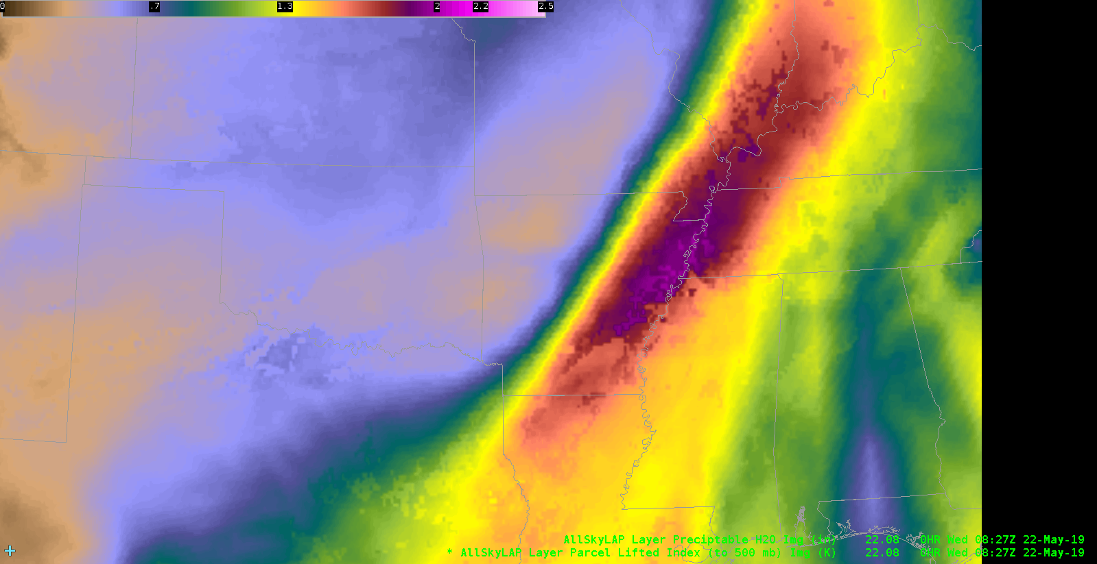
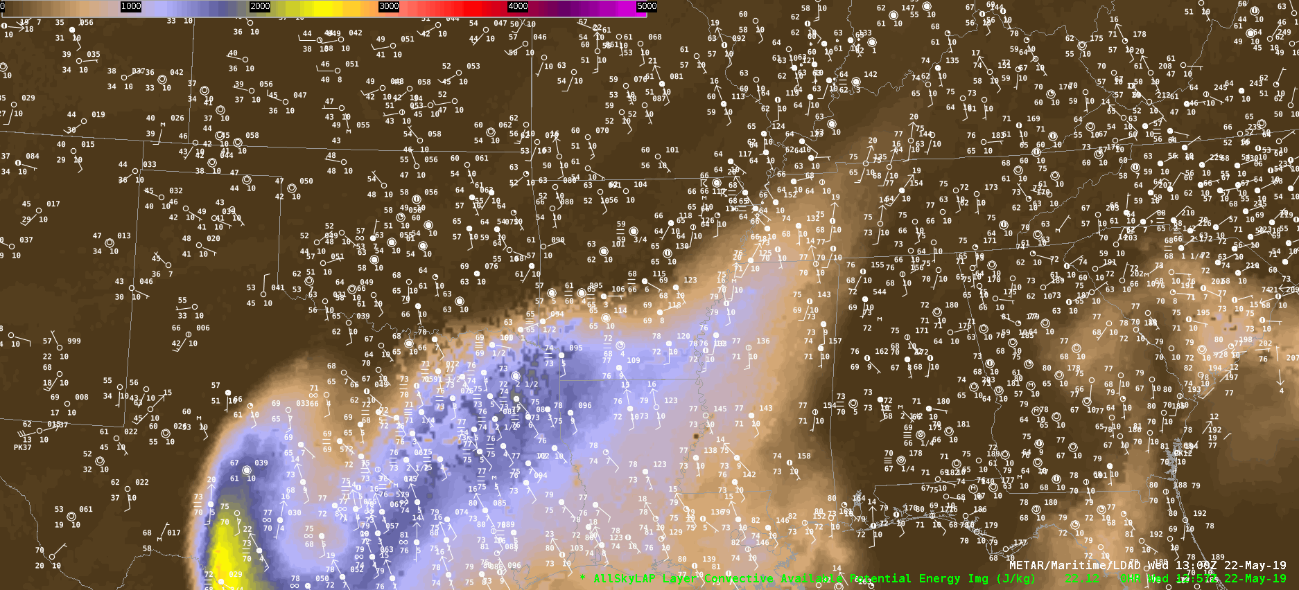
With convective initiation just starting, I wanted to to a comparison of the All Sky CAPE with the SPC mesoanlysis of SBCAPE and MLCAPE. Let’s start with the SBCAPE (all images at 19Z on 5/22).
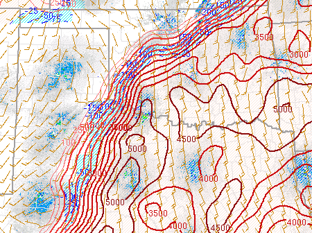
A very sharp gradient in SBCAPE can be seen in the mesoanalysis above, with values ranging from essentially nil in the northwestern part of the state to values over 4000 J/Kg in the southern third of the state.
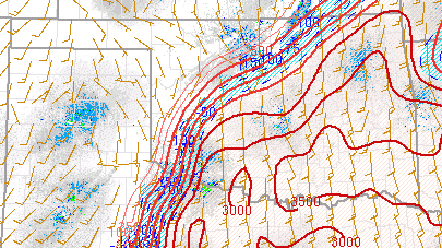
The MLCAPE, as one would expect during maximum surface heating, is somewhat less, with values greater than 2500 J/kg running roughly from Tulsa to Norman, and values in excess of 3500 J/kg along the Red River.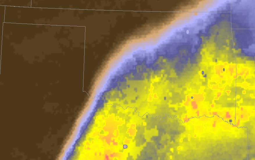

Finally, let’s look at the All Sky CAPE. These values are running about 500 J/Kg lower than the SPC MLCAPE in the Tulsa to Norman corridor, and as much as 1000 J/Kg lower near the Red River. However, it does nicely indicate the “shape” of the area that has MLCAPE, and emphasizes the area with the maximum values. This indicates the product is very helpful in a qualitative sense, but specific values need to be used with caution.
Thorcaster


 -64BoggsLites