AzShear – Increasing Vorticity Along RFGF

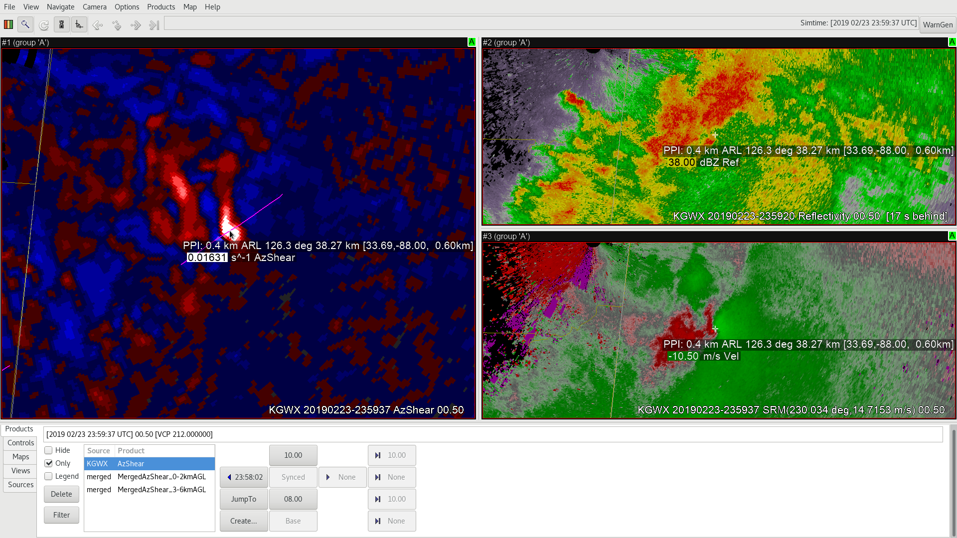
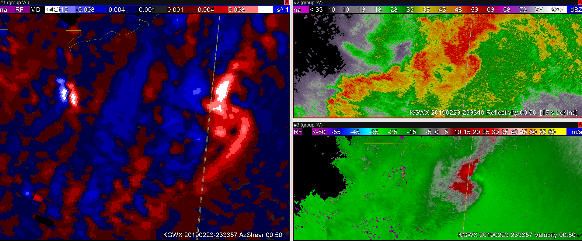
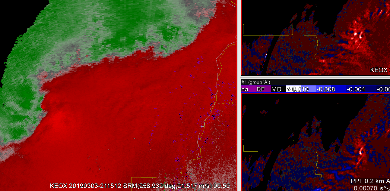
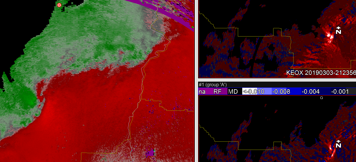
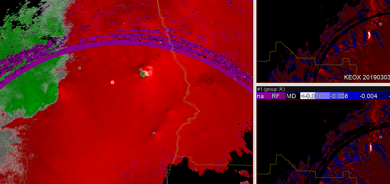
AzShear in this example, highlights the areas along the RFGF where vorticity is increasing, and eventually where the new tornadic circulation forms in several minutes. Something like this may be more identifiable in a radar looped image (especially with SRM), but in a still image a radar velocity scan may not be as intuitive.  In this instance, we see the AzShear output reduced after the previous tornado dissipates through occlusion…

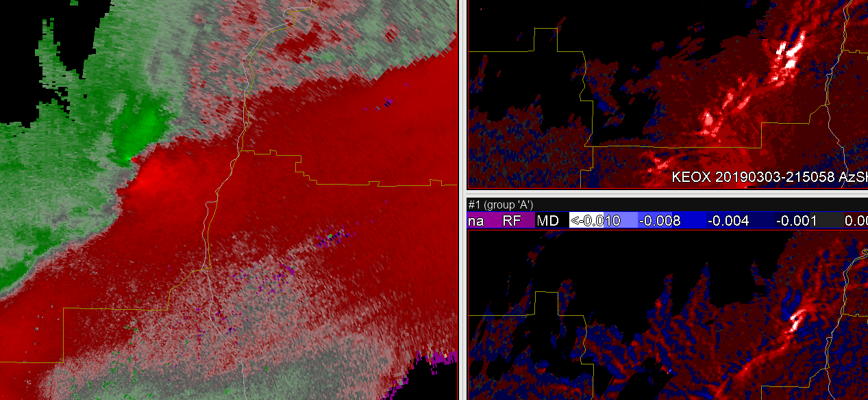
But in the following image (at 2343 UTC) AzShear has already increased to ~0.015…

Tornadogenesis then occurs roughly 8 minutes later  (at 2351 UTC), with an AzShear value of ~0.016. Not much of an increase from the values 8 minutes earlier when GateToGate Shear was not present at the time.

Other thoughts…

  • Long Term potential… Initial values of 1-D pseudo-vorticity is useful as base information, but values can mean different things at different elevations and distances from the radar. Would there be a way to eventually incorporate this information with AzShear for Climotological Tornadic Probabilities? Could help with ProbSVR model…
  • Seems to handle noise relatively well, but certainly still shows waviness in the stable regions. Curious how this might preform in messier situations with surrounding precip. Merged AzShear handles much better than the base, but lag is a downfall.
  • More experienced forecasters may use it well as initial checks, but oversimplification from a 1-D perspective may not translate as well to more inexperienced users. For example,  some less experienced users may equate the color white with a definite tornado, and non-white to no tornado. IDK… probably more of a communications issue unrelated to the product value.
  • Would like to see how this performs in a more marginal case. for instance, some EF-0s within a QLCS.
  • Has the potential to be a dangerous in areas of sidelobes! Perhaps a filter with Reflectivity may be helpful in these situations


#ProtectAndDissipate

AzShear Introduction – Feb 23 Case Study

The introduction to the single-site AzShear product as a broadcaster was exciting. The Mississippi case study was a good one to jump in with! Stepping through the data using AzShear, vel. and the refl data for the storm was very helpful. On most frames, the centroid of the AzShear maximum (or at least the visual maximum created through the colortable, with all values above 0.1 colored white), is right where I’d put the center of circulation using velocity.

This was confirmed when the observed tornado tracks from the survey were overlayed (purple) onto the data as seen in the image above from 2325Z.

A couple things jumped out to me in this analysis of this case study:

  1. The AzShear values do drop a noticeable amount when the eastern Mississippi tornado lifts….which you’d expect both mathematically and conceptually given the gate to gate shear decrease as the velocity couplet deteriorates between 2329 and 2331Z after occlusion. (Note: tornado occurred with southern couplet – no tornado occurred with northern couplet strengthening between 2329 ans 2331Z)


2. In between the eastern Mississippi and western Alabama tornadoes, the AzShear values to return to +.01 and higher, prior to the second tornado occurring and velocity couplet signatures not looking as obvious as when the tornado is on the ground.

3. Is there value to seeing the data differences above .01? Colortable seems to indicate there isn’t, I’m sure published research exists regarding the importance of the values and the colortable choice.

-icafunnel

AzShear RFGF – Occluded Supercell

One unique advantage of the AzShear product I noticed (outside the initial 1-D vorticity analysis) was it’s ability to distinguish gust front boundaries very easily. In this example, you can easily distinguish the FFGF, the tornadic circulation, and the RFGF very quickly and can identify the supercell to be occluded with the RFGF pushing out away from the storm and is cutting off the low-level inflow into the storm. Sure enough, shortly after the supercellular circulation occludes, the tornadic circulation weakens and soon dissipates. In operations, this could be information easily identified by the forecaster noting the tornado may dissipate shortly.

#ProtectAndDissipate
First All-Sky Experience

Interesting CAPE value drop off

During the first opportunity to sit at AWIPS-II and familiarize myself with the different datasets to be evaluated during the EWP, I noticed an interesting drop off of CAPE values from the All-Sky suite.

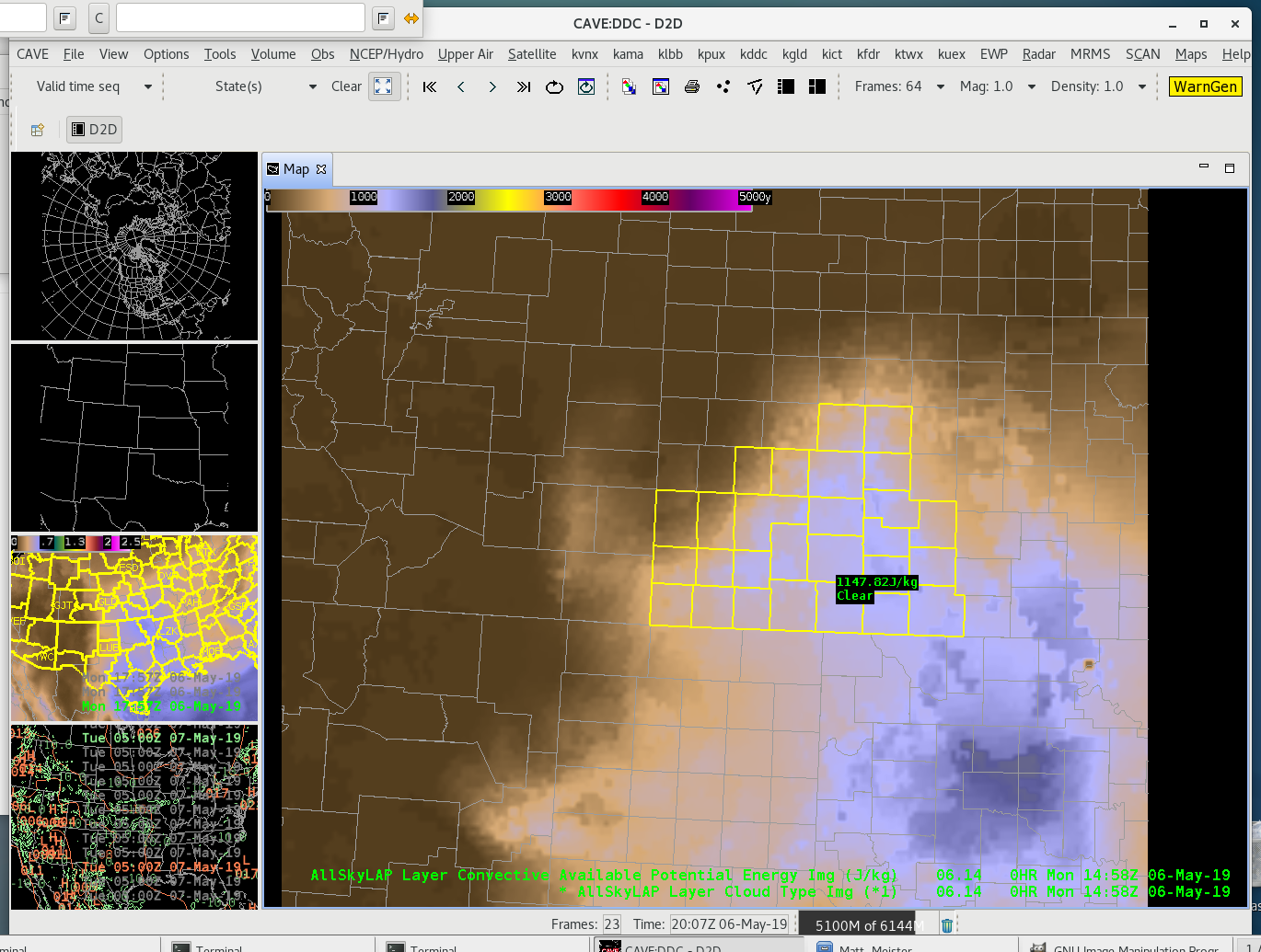
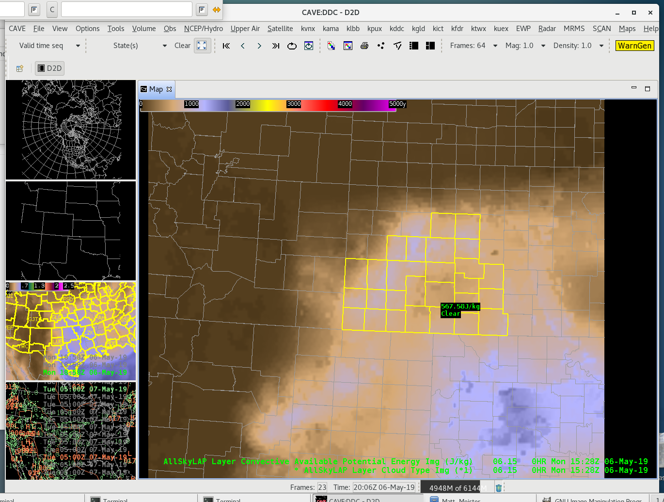
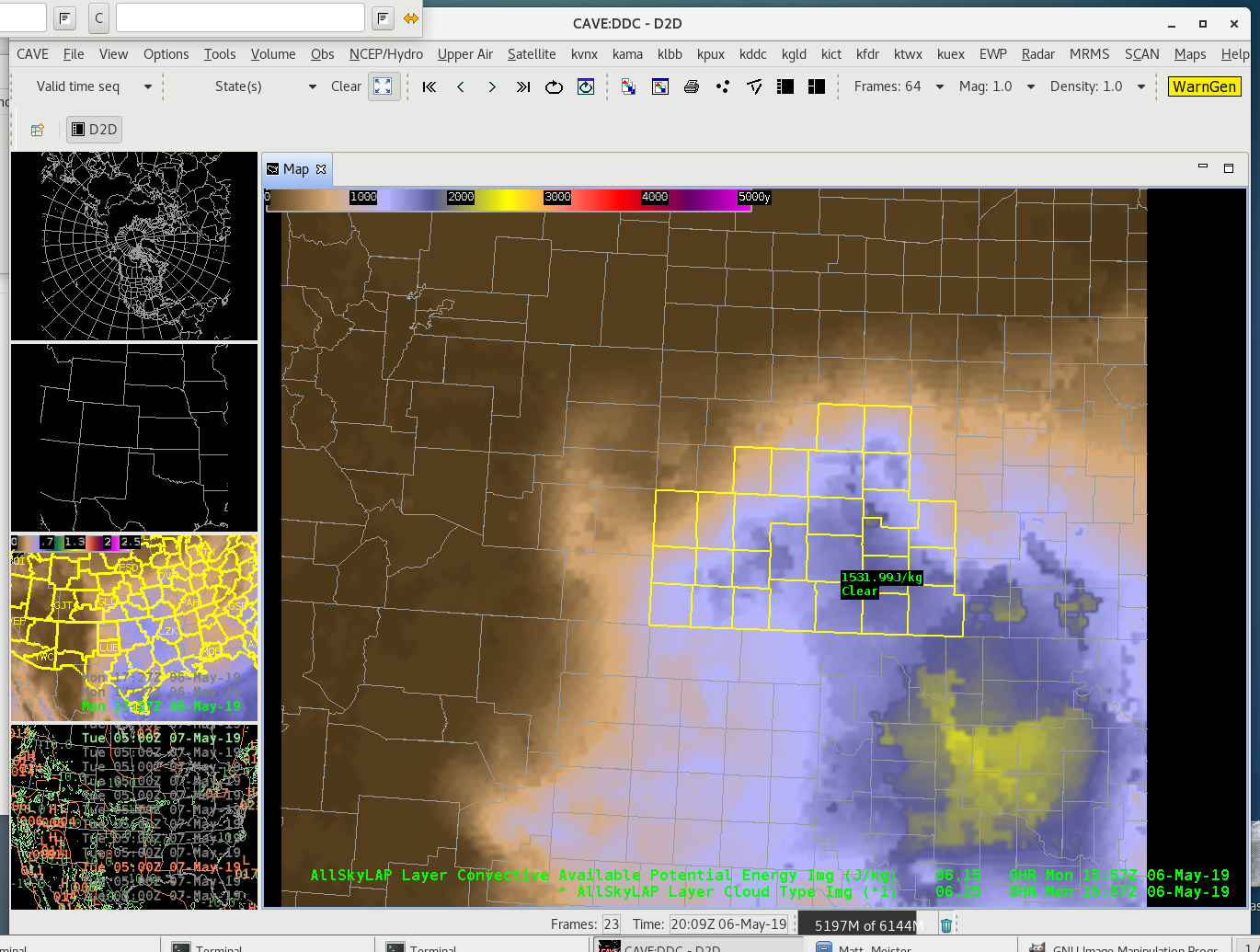
Over the course of an hour, the All-Sky CAPE values oddly drop off by about 2/3 betweem 1458Z and 1528Z, only to rise again in the next frame available at 1557Z. While understanding that atmospheric conditions, such as a propagating storm could cause a drop, analysis of the morning doesn’t indicate the presence of such conditions.

All-sky CAPE values over southwestern KS, 6May2019 1458Z
All-Sky CAPE values over southwestern Kansas 6May2019 1528Z
All-Sky CAPE over southwestern Kansas 06May2019 1557Z

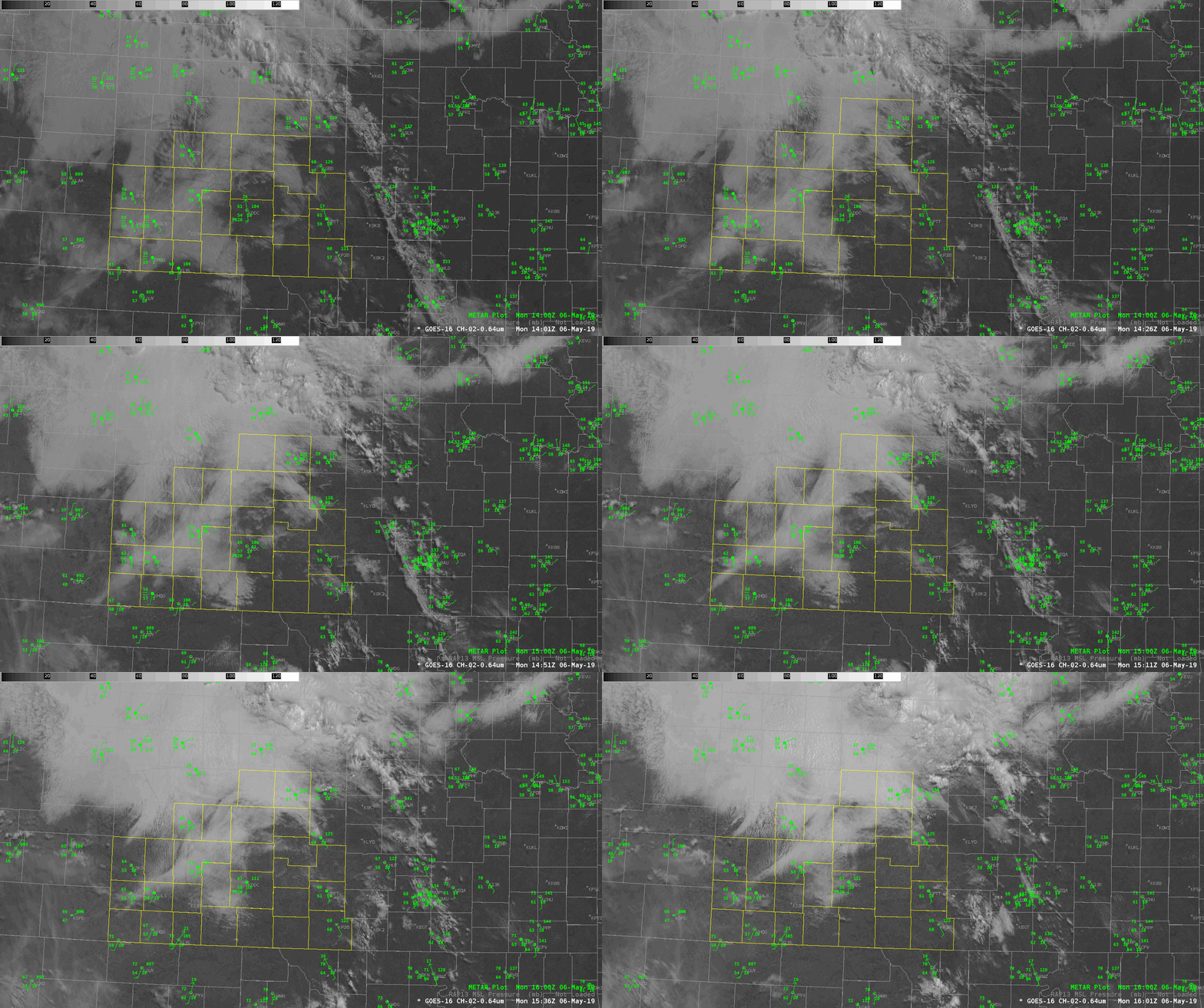
A visible satellite loop of the 0.64 micro channel from GOES-16 shows early morning stratus dissipating between approximately 14-16Z. During this time, the stratus burn off is indicative of the boundary layer beginning to mix out with the sunshine and surface plots corroborate with warming temperatures.

As I’m unable to find anything meteorologically that would support the CAPE drop and rise over 60 minutes, it’s a little concerning as a forecaster too see a jump like this the first time using it. I thought this would be good to point out as a first blog post.

-icafunnel

Visible satellite and surface observations over southwestern Kansas 06May2019 1400-1600Z

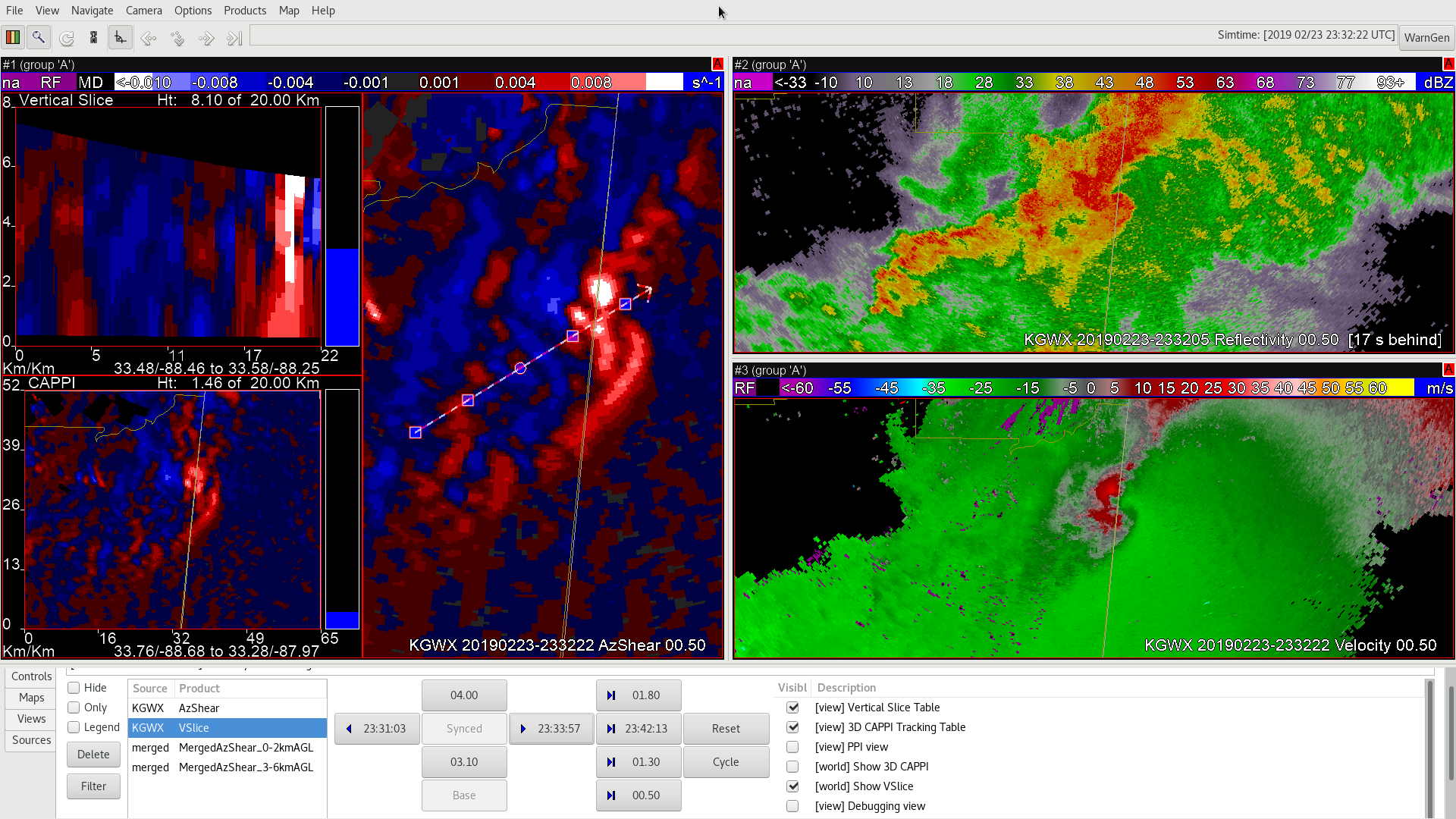
AzShear in “RHI” for Mesocyclone Depth

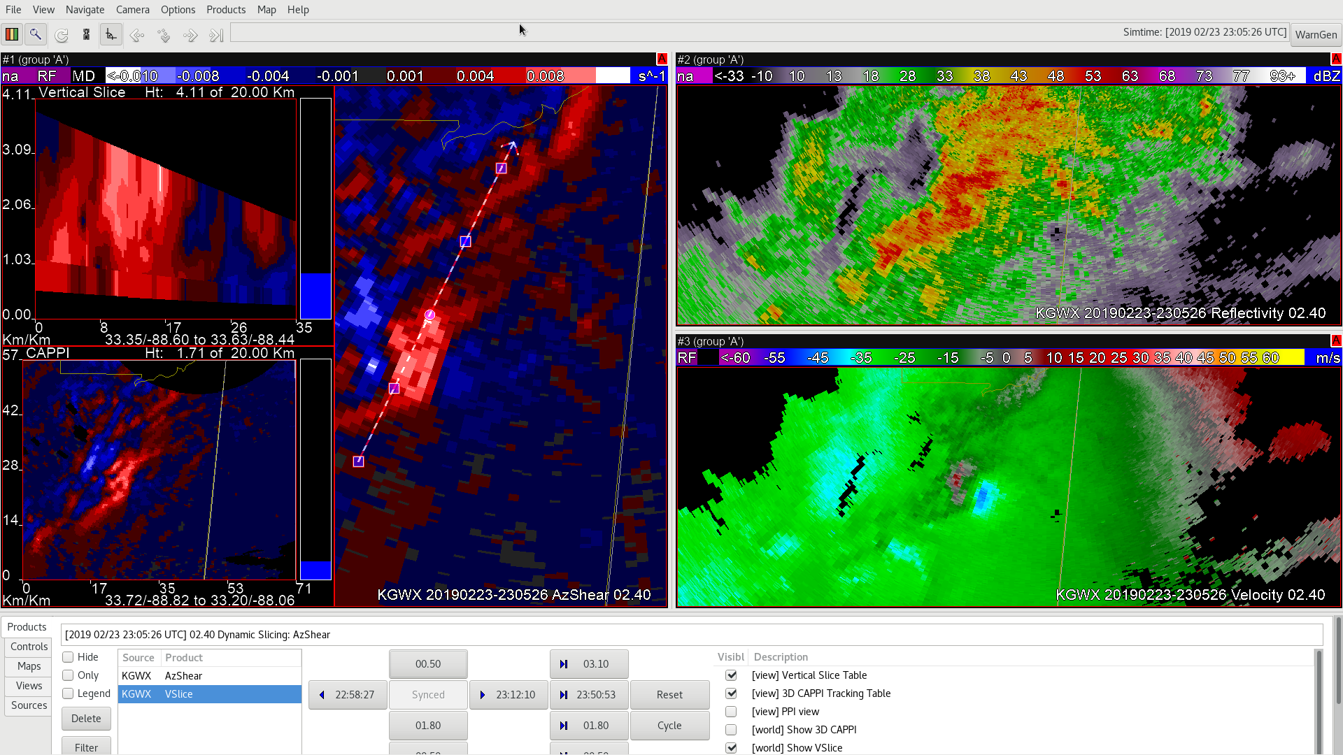
AzShear has the potential to allow for sampling of the depth of rotation in any given storm in time and space to track the evolution of mesocyclones with time.  Before the surface circulation had developed, AzShear was starting to pick up on a strengthening mesocylone at approximately 3km.  Surface velocity products show weak cyclonic convergence starting to develop indicating that the potential was increasing for tornadogenesis sometime soon.  So, what did the time height look like?

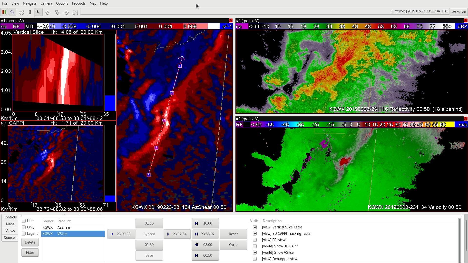
At 23:05:28, the strongest indications in AzShear were at the 2.4 degree tilt in this scan but were rather weak heading down to the lowest tilt (and there is an artifact in the cross section due to a time-matching issue with the SAILS scan).  Not shown is the descending positive AzShear values at or above 0.010 s^-1 with time so that by 23:11:34, the cyclonic shear had now reached the lowest scan:

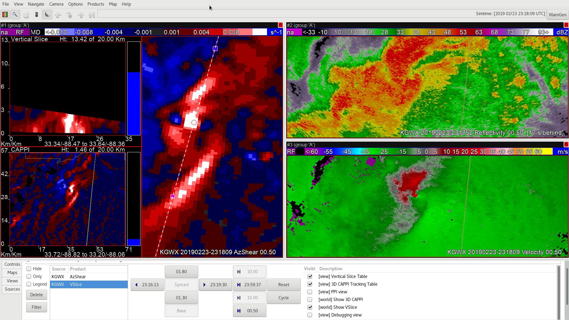
However, the lowest tilt shows that the tornado was possibly still in the process of forming as there was not a strong gate-to-gate couplet yet.  That took another 5 to 7 minutes depending on how strong of a couplet you want.  For this case, we’ll use 23:18:09:

While the strong TVS remained intact, AzShear showed high positive values from the top of the cone of silence down to the lowest tilt.  Once the surface TVS and vortex appeared to have broken down, the mesocyclone aloft was still strong as shown in AzShear at 23:32:22:

This indicates that there is utility in using AzShear in keeping situational awareness of what storms that are rotating are doing with time.  However, the usual caveats apply and YMMV:

  1. Visualizing the 3-D structure using cross-sections will depend on how you place your cross section and how fast the storm is moving with time.  It may be impossible to do 2-D cross sections in 3-D space if the storm is moving fast!
  2.  Since AWIPS doesn’t have 3-D rendering, the ability to accurately “paint” vertical circulations to see overall development is non-existent.
  3. SAILS scans in WDSS-II (and potentially FSI) will not line up with the full Volume Scan so tracking of deep features will be limited at times, also complicating matters.

-Dusty

False High AzShear Values

High positive & negative AzShear values were side by side in an area of drying/sinking air. Operational forecasters will need to keep an eye out for false high values and know when to discard that type of potentially misleading data. This is a good example of why it is still important to never focus on purely AzShear data in a warning environment.

WES Scenario Comments – Quik Trip

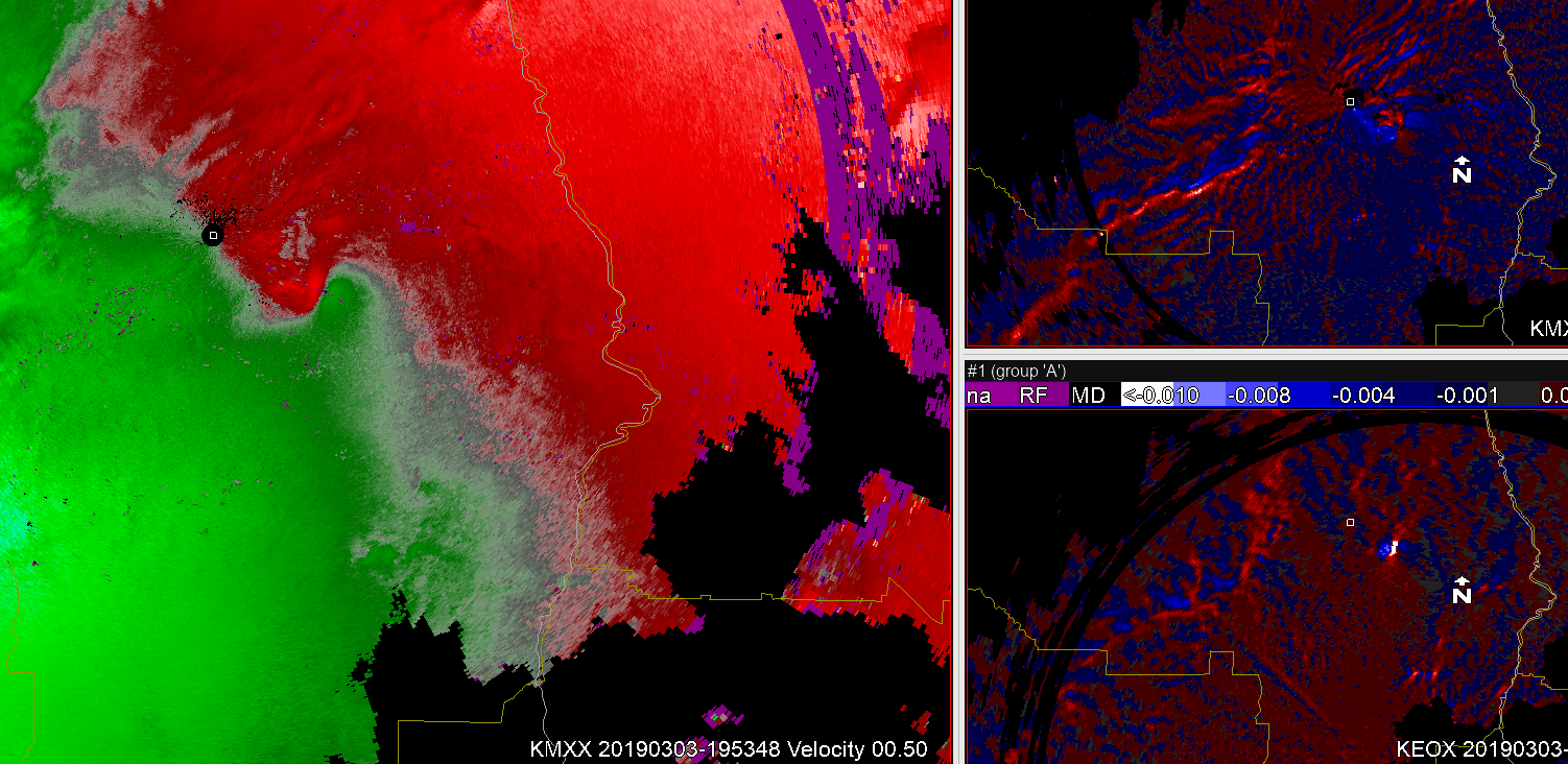
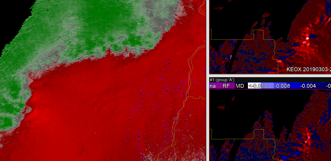
Right off the bat at the beginning of the simulation KEOX AZShear max really jumps out at you!  A great SA example to quickly hone in on area of concern. 0-2 km Azshaer also very good.

Focusing on the squall line upstream, really like the way the elongated max in AZShear draws attention to the increasing shear along leading edge (updraft-downdraft convergence zone UDCZ) of the surging portion of the QLCS.   Often a precursor to MV intensification along the UDCZ. 66

The following sequence shows the evolution of a mesovortex along the UDCZ a little later in the event.  The first panel nicely shows a MV forming (left portion of SRM below) with a AZShear max evident at that location as well. The second panel below suggests that the MV starts to fall back just behind that leading UDCZ while the AZShear maintains a max with that circulation.  What is even more  interesting is that in the 0.5 AZShear in particular, you can still see an elongated area of enhanced shear  associated with the leading UDCZ just downstream from the MV.  You can see these two distinct features even more clearly in the last panel below.  In summary I think the 0.5 and 0-2 km AzShear can hep forecasters identify increasing shear along the UDCZ where it is starting to surge…and then identify subsequent MV development and evolution along the surging UDCZ.

Finally, the image below is several volume scans later showing a very similar sequence as that described above.  A an elongated area of enhance VrShear develops along the UDCZ followed by subsequent MV development.  The MV below in the SRM image is appears to be very likely tornadic at this time.  The 0.5 AzShear (lower right) shows the enhance VRShear with the tornadic MV falling behind the leading UDCZ…and a continuation of the elongated enhanced shear along the surging UDCZ.  This case demonstrated to me that the AZshear can certainly enhance the warning decision makers SA for more quickly identifying line surges and subsequent QLCS MV development.  Given QLCS MVs tend to form in the  around 2 km or so, the 0-2km Azshear product may be of added value to identifying the area of enhance shear a bit sooner perhaps providing a bit more lead time on possible tornado warning –  Great Case! – Quik Twip.

Tags: None

Good non-severe storm with agreement from radar/satellite products

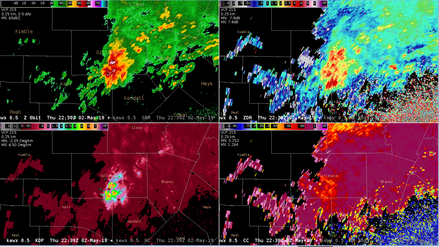
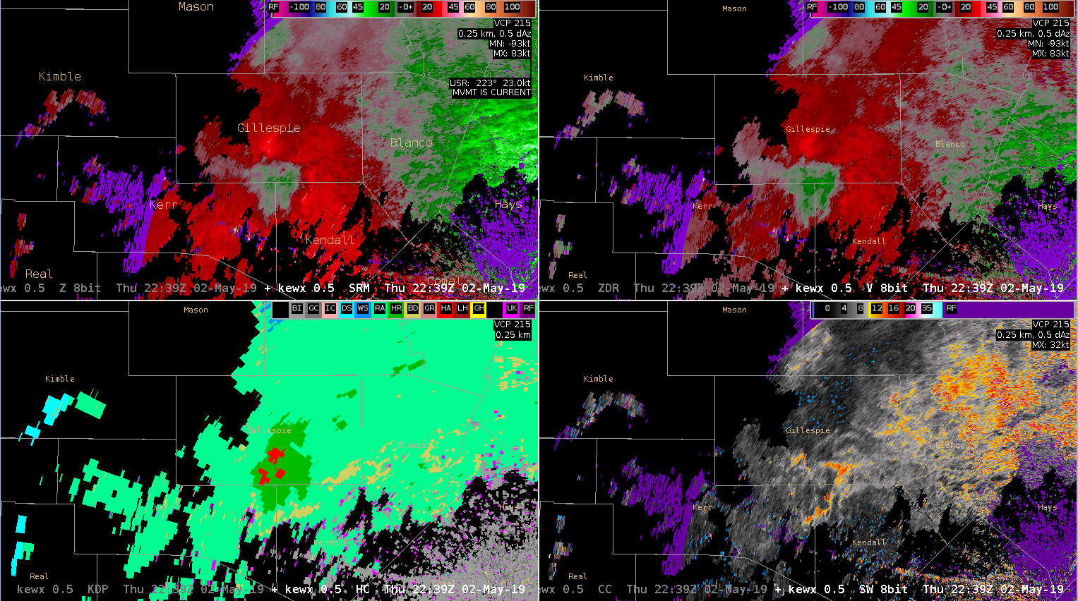
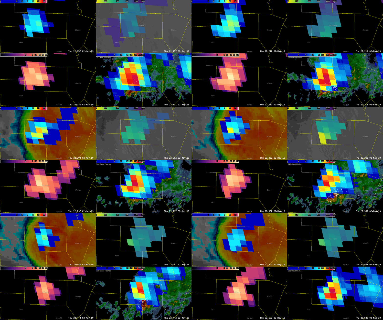
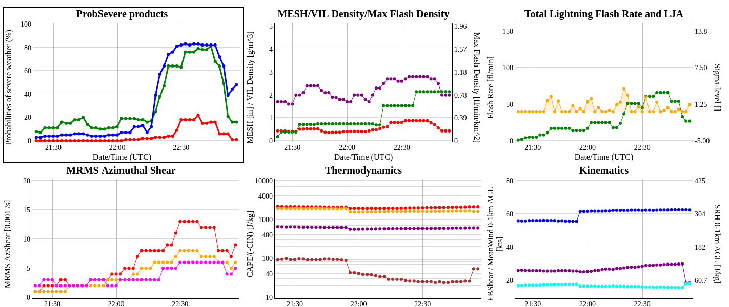
One storm became near severe around 545 pm in EWX CWA. All parameters; lightning, ProbSevere and Dual-pol radar agreed on the evolution of the storm and expected impacts. Radar data suggested there to be equal wind and hail threat based on high ZDR and KDP within the core suggesting sub-severe hail. There was some notching in the back side of the storm’s reflectivity as the front end of the storm surged eastward suggesting some wind threat. Lightning over this time had increase from 10 fl/min to 20 fl/min about 15-20 minutes prior to the development of some weak mid level rotation. As the storm cycled and weakened, so did the lightning and ProbSevere values. An uptick in GLM event density was followed by a slight increase in ProbSevere values toward the end of the loop.

KEWX 4-panel – Refl (UL), ZDR (UR), KDP (LL), CC (LR)

KEWX 4-panel – SRM (UL), V (UR), HC (LL), SW (LR)

GLM sequence of Gillespie County storm – 1-min(FED)(UL),AFA(UR),TOE(LL),EventDensity(LR)

ProbSevere time trends from http://cimss.ssec.wisc.edu/severe_conv/plots/PSplots.php?ID=176047

— SCoulomb