We’ve been monitoring a boundary on both the KEOX and KEVX radar, likely associated with weak surface convergence per surface obs. 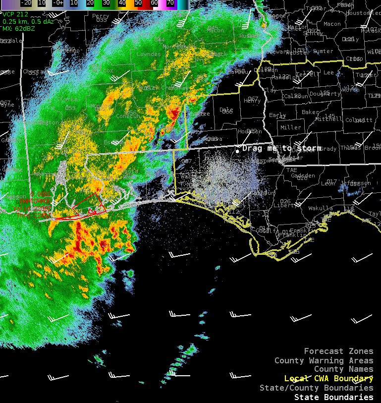
 The layered TPW product shows a tongue of moisture approaching the region. It looks like a line of towering cumulus developed over the Gulf of Mexico as this moisture interacted with the convergence line.
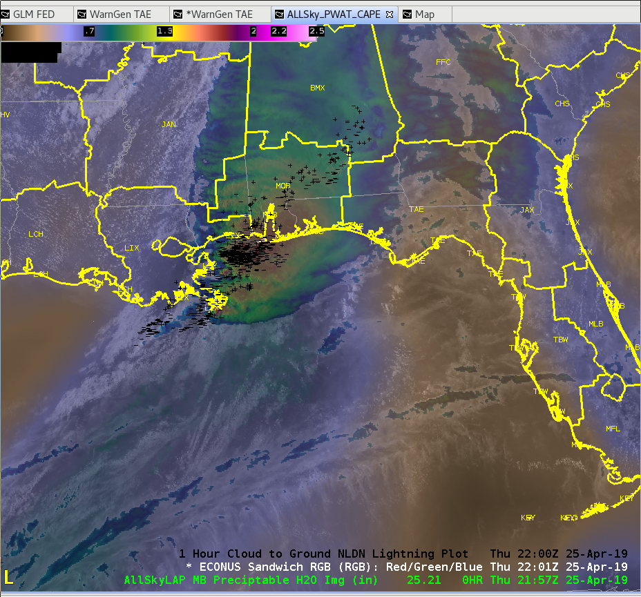 Sandor Clegane
Category: News
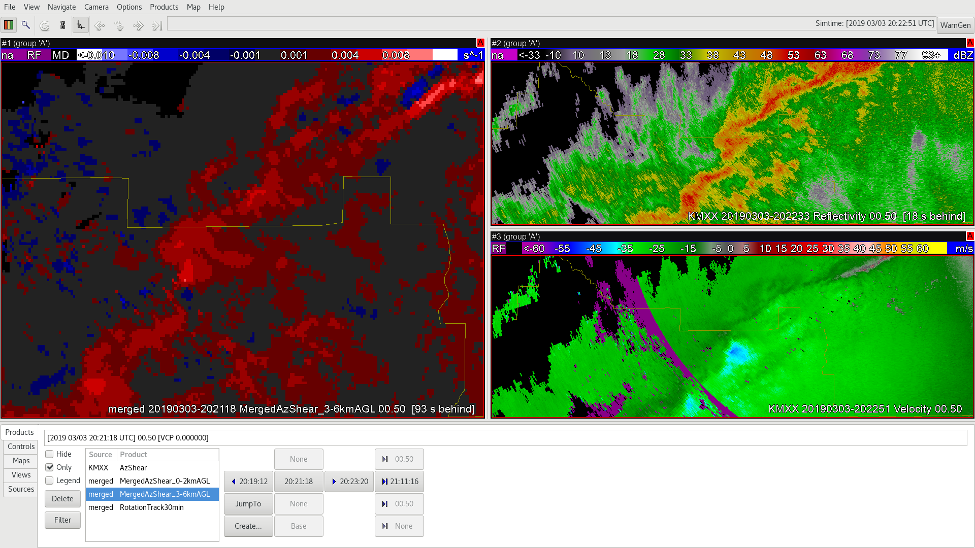
Tracking Meteogram Tool With AzShear
![]()
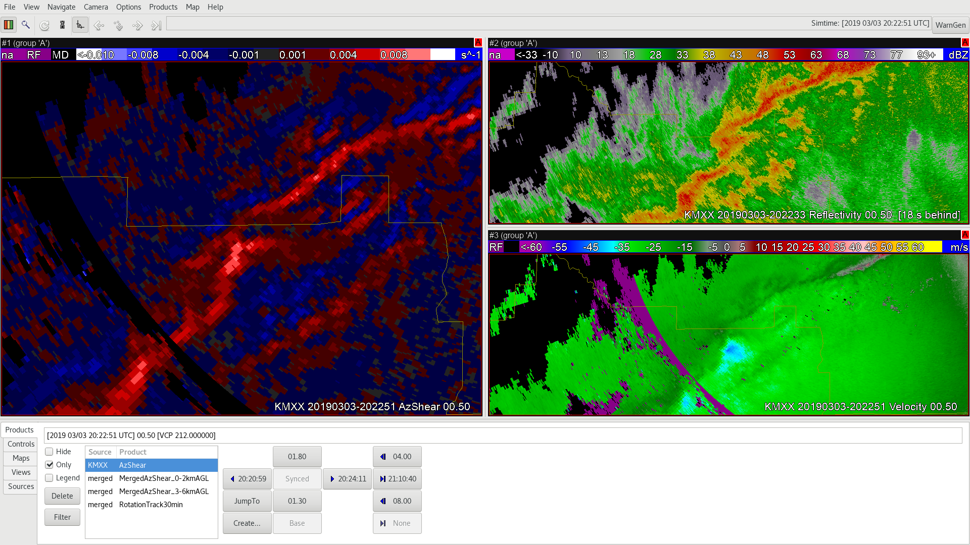
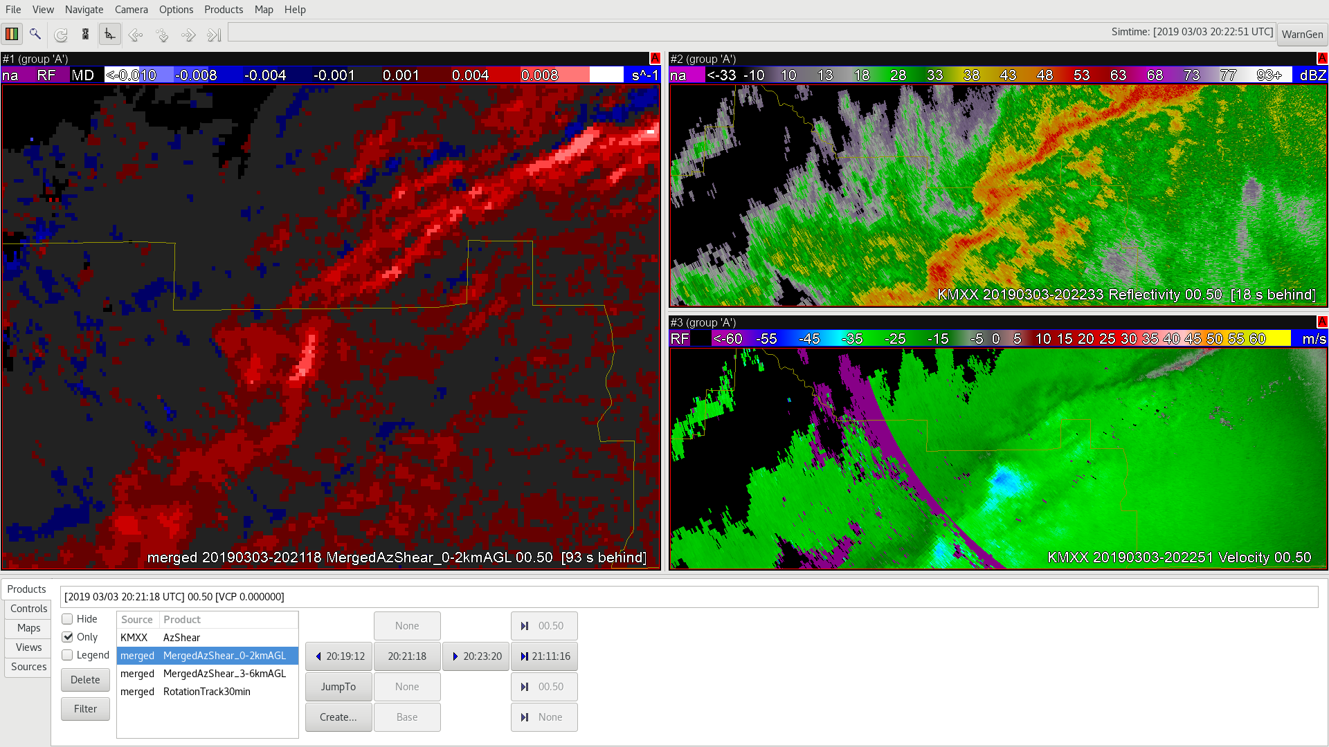
One of the discussion points that has come up about the Merged AzShear product is monitoring the trends of the AzShear as storms progress. One way to do this that is built into AWIPS is the Tracking Meteogram tool. The following are a GIF and PNG for a MCV just off of the MOB CWA. The radar image is above. The GIF shows the tracking tool and AzShear and then the plot showing the trends. In this case you can see general increase in AzShear values. There are some limitations of the Tracking Meteogram took like only being able to track one feature at a time, there is a lot of things to edit and modify with the Meteogram (the position and size of the tracking area), and this would not be an easy tool to modify and update while trying to focus on other warnings.
![]()
![]()
-Alexander T.
Merged AzShear for Strength Trends
An example where AzShear data can show storm trends in one image without looping. As SAILS cuts come in you’re able to view rotational strength trends before the entire image is replaced by the next volume scan. Although this image is looping you can see the times when sails cuts would be overlain on one image.
THE 3 MARCH 2019 CASE FOR AZSHEAR – #4
Below, here’s a snapshot of an example where AzShear isn’t applicable as compared to using it in other situations. This feature is about 66 miles from the radar.
~Gritty
NMDA Struggles To ID Mesocyclones On QLCS
A severe thunderstorm pushed through the northern portion of the CWA and I had a tornado warning in effect in anticipation of tornadoes along the eastern most portion of the bowing line. Unfortunately, the NMDA was not initially identifying mesocyclones along that portion of that line. It was only until well after the warning was issued that the NMDA identified anything along that portion of the line. Sandor Clegane
GLM Assist In DSS
The below image shows GOES-16 day cloud convection (DCC) beneath GLM Minimum Flash Area (MFA). Point F is a DSS event. DCC shows clouds glaciating a county upstream of our DSS event, with the storm becoming electrified shortly after glaciation per MFA. This prompted a call to the emergency manager providing support for the DSS event letting them know that lightning was imminent.
ENI total lightning also shows lightning (white points), but the point data fails to show the extent of the lightning, which may lead decision makers to think that they have more time to react to the approaching lightning than they actually do. Sandor Clegane
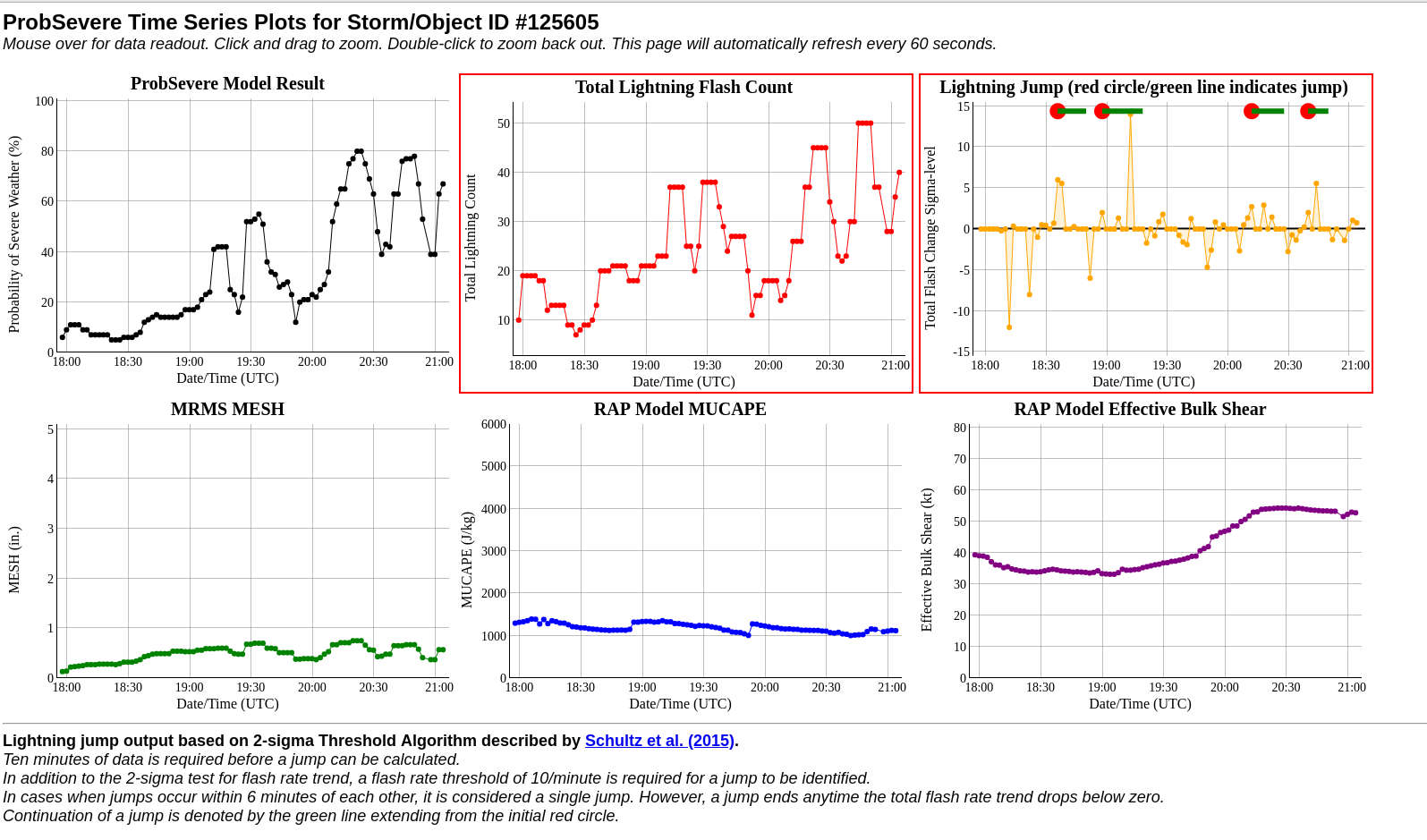
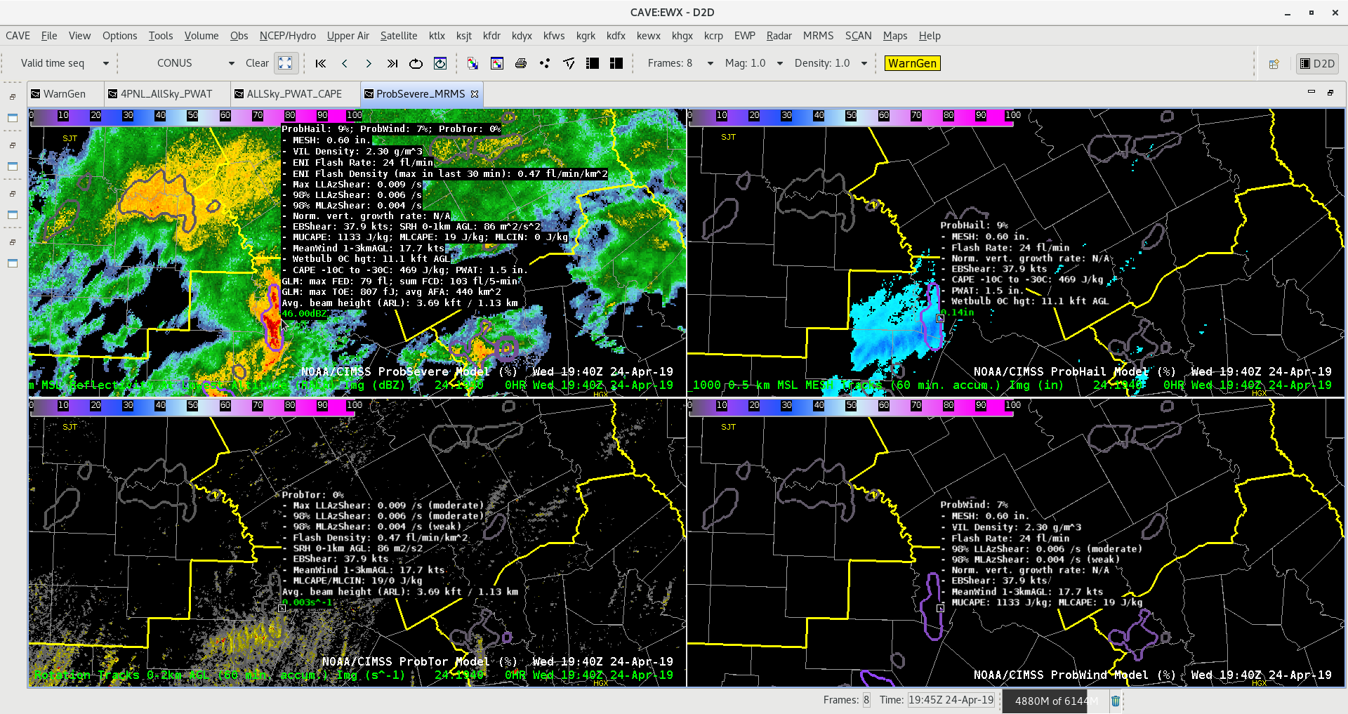
ProbSevere Trend Tracker
ProbSevere has been very useful over the years. One desirable feature would be to have a “trend tracker” see the example from WFO MPX. It sounds like work is being done on this endeavor?
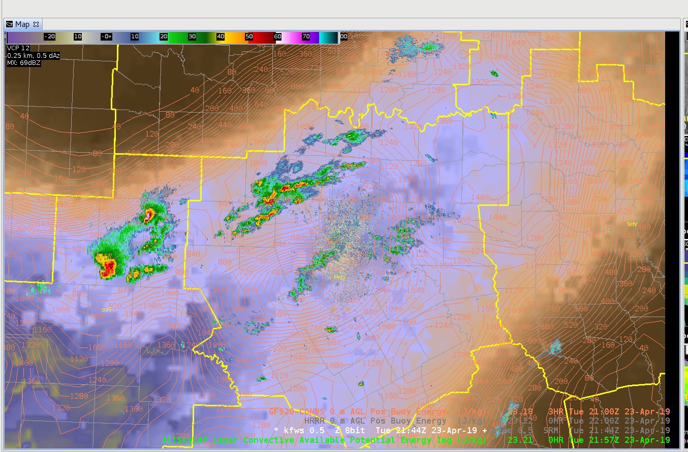
AllSkyLAP CAPE – Trends
Noticed the trend of AllSkyLAP – CAPE was interesting – and bucked the trend of the GFS background.
2157 UTC: LAP seemed to have a good handle on higher CAPE trends at this timeframe with over 1000 J/kg in a wide area – which seemed to match convective trends.
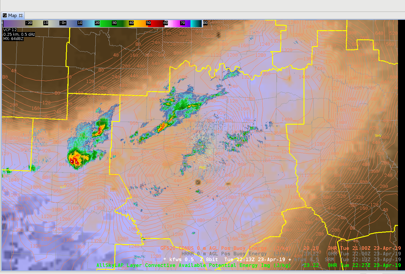
2227 UTC: LAP reduced CAPE over much of the area – even in areas that did not see storms. Skies were generally were generally partly/mostly cloudy – but the trend appeared to reduce values too quickly.
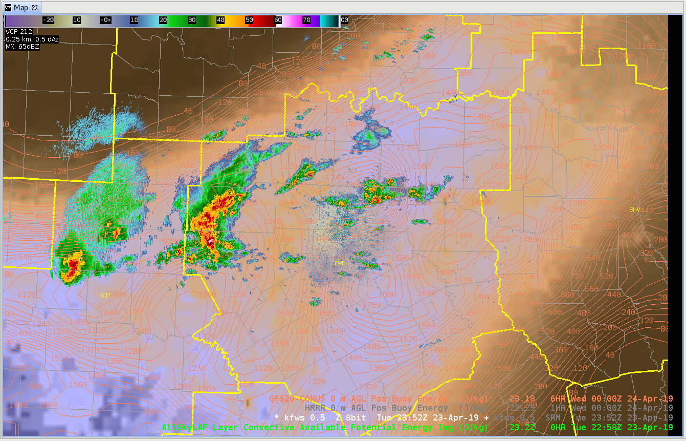
2258 UTC: LAP CAPE appeared boost again somewhat – but still less than the GFS CAPE. These sort of “bouncy” CAPE trends will be examined the remainder of the week – to see if this trend continues.
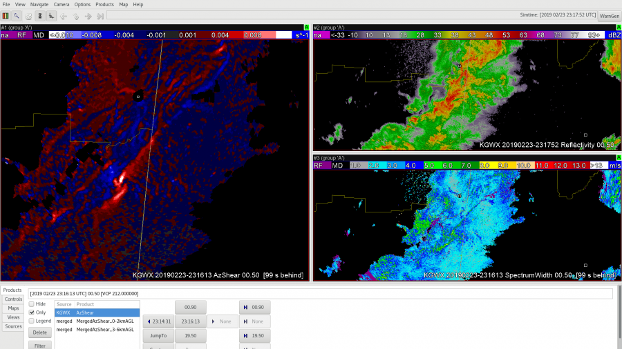
AzShear and the Leading Edge
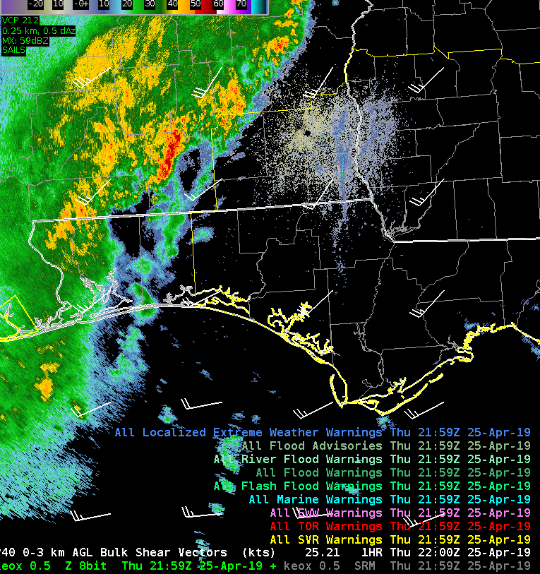
Spectrum Width is (I feel) a seldom used and/or misunderstood product, but one of the uses of it is to view the leading edge of a gust front with messy reflectivity. I think the Az Shear product, especially the single radar version, adds an additional layer to this boundary identification. A forecaster would need to be aware where the radar is with respect to the leading edge as the Az Shear flips whether you are north or south of the radar, but putting the Velocity, SW, and Az Shear together makes that leading edge ID easy. This is important when doing DSS for events for example, identifying and timing out right where the leading edge winds begin. Below are two screenshots one with AzShear, Reflectivity, and SW, and another with AzShear, SW, and Velocity. You can see where the leading edge is in the most norther part of the line in reflectivity (tight gradient that lines up well with SW). In the middle of the reflectivity though it gets messy. While details of the leading edge are still visible in SW, they stand out well in the AzShear, including where a kink the line and a new circulation is developing.
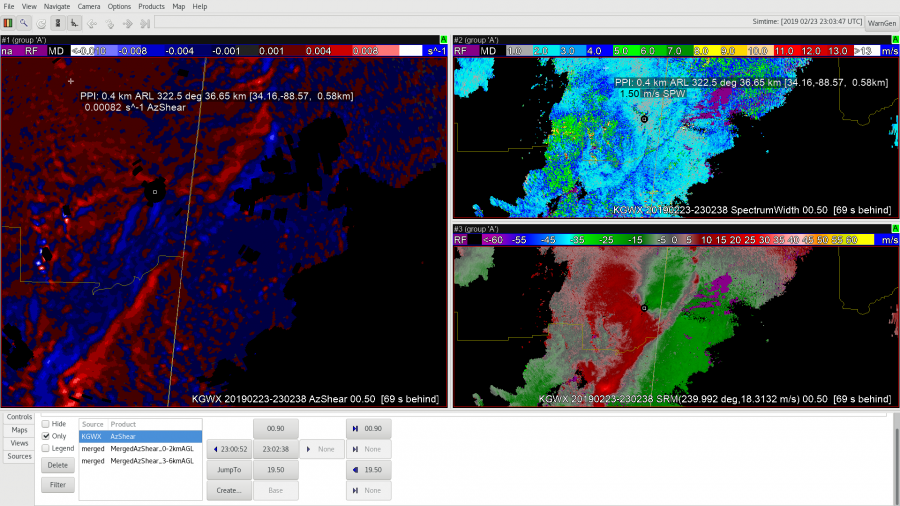
You can see this leading edge of the line in Storm Relative velocity as well (see above). Whether it is for tornadic circulation identification (which SW can also play a role in – high values of Spectrum Width = high turbulence like you’d see around a tight couplet) or for identification of the leading edge of the winds I think a 4 Panel of Reflectivity, Spectrum Width, Velocity, and Single Radar AzShear would be useful and valuable.
-Alexander T.
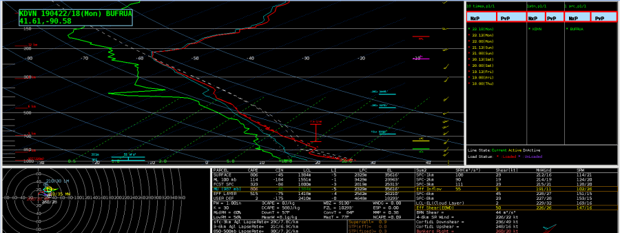
Comparing RAOB to NUCAPS and AllSky Layer Precipitable Water
Davenport launched an 18Z balloon, which gave me the opportunity to compare the RAOB with a NUCAPS sounding (first and second images below, respectively). Initially, I attempted to modify the sounding in NUCAPS to try to bring it closer to the observed values, but after several minutes and attempts at doing that, I realized that I’d have to do multiple levels of modifications before it came anywhere close to the observed sounding. As great as it is to have the ability to modify the NUCAPS sounding, my initial thoughts are that I’m not sure how feasible it would be to do this in a much quicker-paced operational setting. If I’m sitting in the mesoanalyst seat during a severe weather event, I’d need to be able to analyze the available data much faster than doing a more detailed modification would allow.
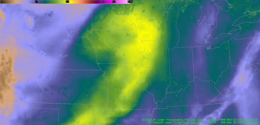
I was also able to do a PWAT comparison between these two soundings and the AllSky Layered Precip product. The NUCAPS and RAOB are very close together in values, whereas since the AllSky product (last image below) is currently utilizing the GFS to fill in the data in the DVN area, it’s noticeably higher (RAOB: 1.0″; NUCAPS: 1.1″; AllSky: 1.3″). I am very happy to be able to underlay the data type for the LAP products, since this is crucial for me to be able to see where the data is coming from and how to correctly assess and apply the right bias adjustments, as necessary.
As for the AllSky Layered Precip product, in general, this is very helpful to be able to identify potential atmospheric rivers and quickly diagnose PWAT trends with a decent degree of confidence, when again combined with the knowledge of what data is being used to compute the output.
~Gritty