

Thunderstorm over northwest Mason county ?is showing Updraft Velocities of 23 meters/sec and maximum vorticity values approaching 17 s-2. Radar shows outflow boundary is moving southeast and should impact the storm by 2140z. Expect storm will continue to increase in intensity. Hovis/Nunez
SJT: EM Discussion @21Z
Location: Latest guidance supports continued development of strong to severe thunderstorms moving across McColloch, San Saba, Llano, San Saba and Mason counties.
Impacts: primary impact will be large hail and damaging winds. there is still potential for isolated tornadoes.
Met discussion: OUNWRF showed evidence of moisture convergence on the h8/h7 wind and theta E H8-7 layer; MRMS Max hail size estimated 1.5″ hail; UAH CI strength of signal showed 80-100 values over the areas of favorable moisture convergence; CI-CTC projected new development over Llano county.
WFO SJT
Outlook – 7 May 2012
The 2012 edition of the Experimental Warning Program’s spring experiment, or EWP2012, kicked off today. We want to welcome our first set of visiting forecasters: Ryan Barnes (WFO, Norman, OK), Jeffrey Hovis (WFO, Charleston, WV), Roland Nuñez (CWSU, Houston, TX), and Andrea Schoettmer (WFO, Louisville, KY).
Today, the forecasters are becoming familiar with how to access the various experimental products and loading and building new procedures. Currently, an MCS is underway in SC Texas, and we have localized to both San Angelo, TX (KSJT) and Austin/San Antonio, TX (KEWX). The SPC DAY1 outlook shows the approximate area of concern (probability of severe hail shown below).

Greg Stumpf, EWP2012 Week 1 Weekly Coordinator
EWP2012 Welcome!
We are in the process of getting the final preparations ready for the EWP2012 spring experiment. Like in 2011, there will be three primary projects geared toward WFO applications, 1) evaluation of 3DVAR multi-radar real-time data assimilation fields being developed for the Warn-On-Forecast initiative, 2) evaluation of model performance and forecast utility of the OUN WRF when operations are expected in the Southern Plains, and 3) evaluation of multiple CONUS GOES-R convective applications, including pseudo-geostationary lightning mapper products when operations are expected within the Lightning Mapping Array domains (OK-TX, AL, DC, FL). We will be conducting EWP2012 for five weeks total (Monday – Friday), from 7 May through 15 June (Memorial Day week excluded).
New for this year, we will be conducting our operations using the AWIPS2 platform. For most of our visiting forecasters, this will be the first time they will use AWIPS2 for real-time operations, and we hope to get some feedback on its utility. Also new for this year, we are going to attempt a “flexible” shift schedule on Tue, Wed, Thu. A the end of the prior day’s shift, we take a look at the Day 2 outlook and forecast models and make a best guess at determining the timing and location of the follow day events. Our flex shifts will begin anytime between 12-3pm and end 8 hours later. This will allow us a better opportunity to catch severe weather events that had peaks outside our normal operating hours in the past.
We’ve “reclaimed” our Mondays as a real-time operations day. In the past, this day was mostly spent providing training and orientation to the visiting forecasters, and if there were any real-time events, we might not have the opportunity to work them. New for this year, the forecasters are taking the training at their WFOs/CWSUs before they arrive in Norman, via a series of self-paced presentations, Articulates, and a WES Virtual Machine case with most of the experimental products included.
Finally, each Friday of the experiment (11 May, 18 May, 25 May, 8 June, 15 June), from 12-1pm CDT, the WDTB will be hosting a weekly Webinar called “Tales From the Testbed”. These will be forecaster-led, and each forecaster will summarize their biggest takeaway from their week of participation in EWP2012. The audience is for anyone with an interest in what we are doing to improve NWS severe weather warnings.
So stay tuned on the blog for more information, daily outlooks and summaries, live blogging, and end-of-week summaries as we get underway on Monday 7 May!
Greg Stumpf, EWP2012 Operations Coordinator
Lightning Jump: 19 Apr 2012 OK & TX
It was an active evening over two of our networks last night, with lightning jumps occurring on multiple storms in OK & TX. SHAVE was active as well though phone numbers in some of the areas were a bit sparse and calling ended at 9pm CDT, with many storm reports appearing just after this. Luckily, storm reports in the region were plentiful including one of 3 in hail SE of Plainview, TX.
Oklahoma (Caddo/Grady Co. storm):

Storm trends, jumps and storm reports (SPC, prelim) for this same storm:

There were multiple other storms in Oklahoma that also had lightning jumps. These storms were along the line from central Canadian Co through NW Oklahoma Co into Logan, Lincoln and Payne Counties. Watching the realtime feed it seems that many of the ‘jumps’ were due to storm mergers along the line. It will be interesting to compare storm cluster size with timing of the jumps in post-analysis. SHAVE did call along this line, but found only dime-to-nickel-size hail.
Plainview, TX storm:
(details to be completed)
—–
SHAVE closeout at Fri 20 Apr 2012 015711 GMT: SHAVE made ~103 calls today. We had 30 hail reports with 2 being severe (1.0″+), 0 being significant (2″+).
SPC storm reports:
http://www.spc.noaa.gov/climo/reports/120419_rpts.html
Lightning Jump – 13 April 2012: Technical Update & Norman Tornado
Earlier entries (to be updated) have gone over a few of the technical issues we’ve found during these first couple of events. Managed to find a new one on Friday.
Our flash sorting algorithm (i.e., w2lmaflash) seems to be having difficulty dealing with timestamps across multiple minutes from multiple domains coming in at the same time. For example, lets say the current time is 2012 UTC… the OK-LMA is sending 2009 UTC data (the more activity the slower the data transfer gets, up to about 4 min latency), but meanwhile there is no activity in the NA-LMA domain so the timestamp on the LDM feed the most recent data is 2012 UTC. This seems to be leading the w2lmaflash algorithm to be ‘prune’ (or drop) flashes that are more than a minute older (our current processing interval) than the most recent time from an LMA network…
At least that’s what I believe the problem is right now since it’s not reproducible in post-processing when it pulls from all the networks at the same time.
—-
I pulled all the data from Friday off the realtime feed and re-ran it over the weekend over the Oklahoma domain. The Norman tornadic storm is labeled as Cell 1 in all the figures and tables below using scale 1 from the w2segmotionll (kmeans) storm tracking.
The total flash rate (TFR) rate for this storm peaked at 282 flashes per min at 2244 UTC, with jumps occurring at 1835, 1844, 1853, 1940, 1952, 2012, and 2027 UTC (Fig. 1). Hail times from Local storm reports associated with this storm were recorded at 2041 (1 in), 2055 (1 in), and 2142 (1.5 in). The EF1 tornado moved through Norman, OK between 2102 and 2113 UTC (estimates from TDWR).

I’m discounting the lightning jump at 2012 UTC since there was no real-time radar merger between 2000 and 2008 UTC, hence nothing for the algorithm to track. Oddly, during this same time period [2002-2008 UTC] four stations in the OKLMA were also not communicating, leading to too few stations to do any quality control for flash sorting. So it is unknown whether the storm would have produced a lightning jump at this time had the merger/tracking been working correctly.
What is really interesting with this storm is how the character of the lightning changed prior to 2000 UTC and after 2010 UTC as the storm began it’s deviant motion right (towards Norman). The animation below (5 min intervals) catches this character as lightning initiations grow not only in number but also across the storm. The flash rate continues to increase with initiations spreading into the anvil region by the time the core of the storm is over Norman. This increase in flash rate and expanded coverage of lightning is reflective of change in the strength and size of the main updraft core over the same time period (linked via storm electrification processes in around the updraft region).
20120413_animation (quicktime movie, looks a bit better than gif animation below. Either way, you’ll need to click on the link above or image below to see the animation)

There was also a tornado reported in Mustang at 12:45 am CDT, but I haven’t had time to evaluate that storm yet.
Feel free to leave any questions or comments below or send them directly to me at kristin.kuhlman -at- noaa.gov
Lightning Jump: Network Range
Since the LMA networks depend on a line-of-sight for the time-of-arrival detections, distance from the network center is a key aspect to quality control. While accuracy of a any VHF detection in the center of the network is around ~10 m, this drops off dramatically with range. Flash sorting helps to remove some of this dependency, however, we still want to make sure jumps are not occurring simply because a storm is moving into to the LMA domain.
Originally, this network range issue was planned to be part of the flash sorting algorithm, but after looking at the data we decided to change it to a strict 150 km range (Fig. 1). But I was still seeing an effect of storms entering the network, so I decided to reduce the range again to 125 km (Fig. 2).

We’ve now switched to 125 km for the majority of the networks (100 km for FL). This means that if any part of the identified k-means cluster overlaps the region within 125 km of the network center it is eligible for a lightning jump. (And, yes, this does mean that the majority of a cluster can be outside the range, hence why we went a little stricter and confined it to 125 km instead of 150 km).
The new network range map can be seen below:

I don’t have the exact location of the OKLMA southwest extension yet, nor is the data feed working in realtime so that is being left out for the moment.
Lightning Jump – Week 1: 2 Apr 2012 – 9 Apr 2012
Moving an algorithm into real-time operations is full of pitfalls and challenges. This first week of operations for the lightning jump algorithm was no exception. No matter how much archive data you test on, there are certain aspects that change once you’re at the mercy of a real-time feed. Add to that, working with weather data where the outcomes are unknown and you get a great recipe for failure.
This first week we had three events to test data on, with the SHAVE project active on 2 of the days. The below images (screenshots from the event) will give you a chance to see our visualization of the lightning jump for the SHAVE participants and what you can see real time during future events at: http://ewp.nssl.noaa.gov/projects/shave/data/
Basically, the jump is currently being visualized by colored circles along the track of the centroid of the identified storm cluster. When a storm has a lightning flash rate > 10 flashes per min, but does not have an active ‘jump’ a gray circle is placed along the track. When the storm meets the jump criteria, the circle changes to red. The activity this first week was our first chance to see the visualization and get the data over to kml format (Kiel Ortega was instrumental in getting all of this up and going).
–
5 Apr 2012: Northern Alabama
(to be filled in w/ info on any jumps)
SHAVE closeout on Fri 06 Apr 2012 at 011011 GMT: SHAVE made ~471 calls today. Today we had 98 hail reports with 11 being severe (1.0″+), 0 being significant (2″+). We had 1 wind reports today.
SPC storm reports for this event: http://www.spc.noaa.gov/climo/reports/120405_rpts.html
–
7 Apr 2012: Oklahoma

SHAVE was not active on this day and there were no warnings or storm reports over any of the LMA regions.
–
9 Apr 2012: Oklahoma
Activity on 9 Apr 2012 was primarily outside the central range of the OKLMA network, though there was a chance that storms would move into range. I’ve included it here mostly for illustration of storm cluster identification and storm tracking.

The kmeans storm identification works on 3 separate scales, simply thought of small, medium and large (or 1, 2 and 3). Each of these is using Reflectivity at -10 C, with thresholds set such that all reflectivity less than 20 dBZ becomes 0 and all greater than 50 dBZ appears at 50 dBZ to the algorithm. We are also using a percent filter such that pixels nearby that are partially filled or surrounded by pixels that are filled match the neighbors. This acts to expand the cluster slightly, with the goal to pick up more of the lightning flashes. Looking at the example in the screenshot above, all the CG flashes within the colored area would be counted as occurring with that storm, anything outside the area, even closely nearby will not be associated. Sometimes (at scales 1 & 2 especially) this may combine storms that the human forecaster would deem to be separate entities. This is typically a problem with smaller storms occurring in close proximity to each other as we had from this example on 9 Apr.
The corresponding visualization in Google Earth (or similarly on Google Maps) can be seen below.

SHAVE closeout at Mon 09 Apr 2012 234803 GMT. SHAVE made ~109 calls today. We had 27 hail reports with 13 being severe (1.0″+), 10 being significant (2″+)
Lightning Jump Algorithm Test – Welcome
This is the initial “welcome” post for the Lightning Jump Algorithm test. Please come back using the direct link to the “Lightning Jump Algorithm” category for additional posts.
Greg Stumpf, CIMMS/MDL
Precise Threat Area Identification and Tracking Part III: How good can TIM be?
For my presentation at the 2011 NWA Annual Meeting in Birmingham, I wanted to introduce the concept of geospatial warning verification and then apply it to a new warning methodology, namely Threats-In-Motion (TIM). To best illustrate the concept of TIM, I’ve been using the scenario of a long-track isolated storm. To run some verification numbers, I needed a real life case, so I chose the Tuscaloosa-Birmingham Alabama long-track tornadic supercell from 27 April 2011 (hereafter, the “TCL storm”), shown in earlier blog posts, and I’ll repeat some of the figures and statistics for comparison. This storm produced two long-tracked tornadoes within Birmingham’s County Warning Area (CWA).
The choice of that storm is not meant to be controversial. After all, the local WFO did a tremendous job with warning operations, given the tools and they had and within the confines of NWS warning policy and directives. Recall the statistics from the NWS Performance Management site:
Probability Of Detection = 1.00
False Alarm Ratio = 0.00
Critical Success Index = 1.00
Percent Event Warned = 0.99
Average Lead Time = 22.1 minutes
These numbers are all well-above the national average. We then compared these numbers to those found using the geospatial verification methodology for “truth events”:
CSI = 0.1971
HSS = 0.2933
Average Lead Time (lt) = 22.9 minutes
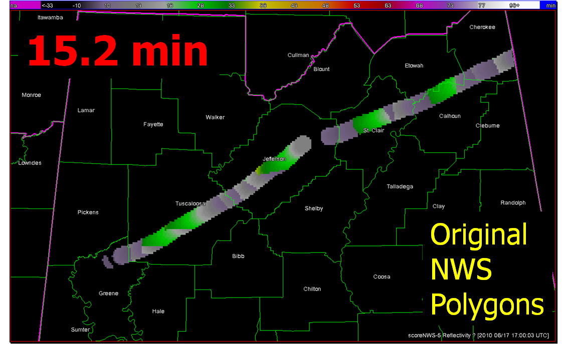
Average Departure Time (dt) = 15.2 minutes
Average False Time (ft) = 39.8 minutes
And recall the animation of the NWS warnings I provided in an earlier blog post:

What if we were to apply the Threats-In-Motion (TIM) technique to this event? Recall from this blog entry that I had developed a system that could automatically place the default WarnGen polygons at the locations of human-generated mesocyclone centroids starting at the same minute that the WFO issued its first Tornado Warning on the storm as it was entering Alabama. I used a re-warning interval of 60 minutes. If you adjust the re-warning interval to one minute (the same temporal resolution of the verification grids), you now have a polygon that moves with the threat, or TIM. The animation:

Let’s look at the verification numbers for the TIM warnings:
CSI = 0.2345
HSS = 0.3493
Average Lead Time (lt) = 51.2 minutes
Average Departure Time (dt) = 0.8 minutes
Average False Time (ft) = 23.1 minutes
Comparing the values between the NWS warnings and the TIM warnings visually on a bar graph:

All of these numbers point to a remarkable improvement using the Threats-In-Motion concept of translating the warning polygons with the storm, a truly storm-based warning paradigm. Let’s also take a look at how these values are distributed in several ways. First, let’s examine Lead Time. The average values for all grid points impacted by the tornado (plus the 5 km “splat”) are more than doubled for the TIM warnings. How are these values distributed on a histogram:


For the TIM polygons, there are a lot more values of Lead Time above 40 minutes. How do these compare geospatially?


Note that the sharp discontinuities of Lead Time (from nearly zero minutes to over 40 minutes) at the downstream edges of the NWS warnings (indicated by yellow arrows in the top figure) are virtually eliminated with the TIM warnings. You do see a few discontinuities with TIM; these small differences are caused by changes in the storm motions at those warned times.
Moving on to Departure Time, the average values for all grid points impacted by the tornado (plus the 5 km “splat”) are reduced to nearly zero for the TIM warnings. How are these values distributed on a histogram:


And geospatially:

With the TIM polygons, the departure times across the path length of both tornadoes is pretty much less than 3 minutes everywhere. Whereas, the NWS polygon Departure Times are much greater, and there are some areas still under the NWS warning more than 30 minutes after the threat had passed.
Finally, looking at False Alarm Time distributions both on histograms and geospatially:


There are some pretty large areas within the NWS polygons that are under false alarm for over 50 minutes at a time, even though these warnings verified “perfectly”. In comparison, the TIM warnings have a much smaller average false alarm times for areas outside the tornado path (about a 42% reduction). However, there are a number of grid points that are affected by the moving polygons for just a few minutes. How would we communicate a warning that is issued and then canceled just a few minutes later? That is food for future thought. I’ve also calculated an additional metric, the False Alarm Area (FAA), the number of grid points (1 km2) that were warned falsely. Comparing the two:
NWS FAA = 10,304 km2
TIM FAA = 8,103 km2
There is a 21% reduction in false alarm area with the TIM warnings, much less than the reduction in false alarm time. The reduction in false alarm area is more a function in the size of the warning polygons. The WarnGen defaults were used for our TIM polygons, but it appears that the NWS polygons were made a little larger than the defaults.
So, for this one spectacular long-tracked isolated supercell case, the TIM method shows tremendous improvement in many areas. But there are still some unanswered questions:
- How will we deal with storm clusters, mergers, splits, lines, etc.?
- How could TIM be implemented into the warning forecaster’s workload?
- How would the information from a “TIM” warning be communicated to users?
- How will we deal “edge” locations under warning for only a few minutes?
Future blog entries will tackle these.
Greg Stumpf, CIMMS and NWS/MDL