

At 1732z…UAH-CI showed a signal strength in excess of 90 and the UW-CTC showed cloud top cooling of -9 degC. Storm did develop in the area where the two values were seen around 1745z and continued thru 1845z. Feel this is a success for both methods. Barnes/Hovis
Author: Greg Stumpf
BRO Starr county update @ 1930z.
Severe storm over northern Starr county increasing in intensity. This can be seen in the maximum updraft product. In addition…Max surface vorticity and Updraft Helicity associated with this storm have been increasing with time. Vorticity (up to 3 km & 3-7 km)(not shown) are also increasing. SRM still not showing any rotation…but will continue to monitor storm. Barnes/Hovis

8 May 2012: Outlook
Looks like we are operating in S and SW Texas again. The upper level flow and shear remains best under the sub-tropical jet, and ample moisture remains in place. Unfortunately, there is no cap in the south Texas area, and convection is already ongoing, with some embedded severe, in that area. Shear is adequate for severe, and a small chance of tornadoes. But there is a lot of current convection owing to the weak cap. And there is a chance for storms to move out of Old Mexico across the Rio Grande. Nevertheless, we are going to have one team operate as Brownsville (BRO) and the MRMS and 3DVAR domains will be available to them over that area. We have a contingency to also add Corpus Christie (CRP) as well if needed.
A second area of convection, with CI just beginning, is over far west Texas and southern New Mexico, as well as adjacent Old Mexico. Moisture is mre lacking in that area, so the main threat will be microbursts. We will have our second team operating as the El Paso, TX (EPZ) office and look primarily at the nowcast and CI products only, since this is too far west to include in the MRMS domain.
Here is the SPC DAY1 outlook for comparison:

Greg Stumpf, EWP2012 Week#1 Coordinator
Daily Summary – 7 May 2012
Our first day for EWP2012 so our teams operating an MCS with embedded severe cells in the San Angelo, TX, (SJT) and Austin/San Antonio, TX (KEWX) WFOs. The storms were moderately severe with low coverage. Mostly 1-1.75″ hail, a few wind damage reports, and one tornado report near Llano, TX. Our teams issued a few SVR warnings, as they were adapting to the new experimental products.

Greg Stumpf, EWP2012 Week #1 Coordinator
Outlook – 7 May 2012
The 2012 edition of the Experimental Warning Program’s spring experiment, or EWP2012, kicked off today. We want to welcome our first set of visiting forecasters: Ryan Barnes (WFO, Norman, OK), Jeffrey Hovis (WFO, Charleston, WV), Roland Nuñez (CWSU, Houston, TX), and Andrea Schoettmer (WFO, Louisville, KY).
Today, the forecasters are becoming familiar with how to access the various experimental products and loading and building new procedures. Currently, an MCS is underway in SC Texas, and we have localized to both San Angelo, TX (KSJT) and Austin/San Antonio, TX (KEWX). The SPC DAY1 outlook shows the approximate area of concern (probability of severe hail shown below).

Greg Stumpf, EWP2012 Week 1 Weekly Coordinator
EWP2012 Welcome!
We are in the process of getting the final preparations ready for the EWP2012 spring experiment. Like in 2011, there will be three primary projects geared toward WFO applications, 1) evaluation of 3DVAR multi-radar real-time data assimilation fields being developed for the Warn-On-Forecast initiative, 2) evaluation of model performance and forecast utility of the OUN WRF when operations are expected in the Southern Plains, and 3) evaluation of multiple CONUS GOES-R convective applications, including pseudo-geostationary lightning mapper products when operations are expected within the Lightning Mapping Array domains (OK-TX, AL, DC, FL). We will be conducting EWP2012 for five weeks total (Monday – Friday), from 7 May through 15 June (Memorial Day week excluded).
New for this year, we will be conducting our operations using the AWIPS2 platform. For most of our visiting forecasters, this will be the first time they will use AWIPS2 for real-time operations, and we hope to get some feedback on its utility. Also new for this year, we are going to attempt a “flexible” shift schedule on Tue, Wed, Thu. A the end of the prior day’s shift, we take a look at the Day 2 outlook and forecast models and make a best guess at determining the timing and location of the follow day events. Our flex shifts will begin anytime between 12-3pm and end 8 hours later. This will allow us a better opportunity to catch severe weather events that had peaks outside our normal operating hours in the past.
We’ve “reclaimed” our Mondays as a real-time operations day. In the past, this day was mostly spent providing training and orientation to the visiting forecasters, and if there were any real-time events, we might not have the opportunity to work them. New for this year, the forecasters are taking the training at their WFOs/CWSUs before they arrive in Norman, via a series of self-paced presentations, Articulates, and a WES Virtual Machine case with most of the experimental products included.
Finally, each Friday of the experiment (11 May, 18 May, 25 May, 8 June, 15 June), from 12-1pm CDT, the WDTB will be hosting a weekly Webinar called “Tales From the Testbed”. These will be forecaster-led, and each forecaster will summarize their biggest takeaway from their week of participation in EWP2012. The audience is for anyone with an interest in what we are doing to improve NWS severe weather warnings.
So stay tuned on the blog for more information, daily outlooks and summaries, live blogging, and end-of-week summaries as we get underway on Monday 7 May!
Greg Stumpf, EWP2012 Operations Coordinator
Lightning Jump Algorithm Test – Welcome
This is the initial “welcome” post for the Lightning Jump Algorithm test. Please come back using the direct link to the “Lightning Jump Algorithm” category for additional posts.
Greg Stumpf, CIMMS/MDL
Precise Threat Area Identification and Tracking Part III: How good can TIM be?
For my presentation at the 2011 NWA Annual Meeting in Birmingham, I wanted to introduce the concept of geospatial warning verification and then apply it to a new warning methodology, namely Threats-In-Motion (TIM). To best illustrate the concept of TIM, I’ve been using the scenario of a long-track isolated storm. To run some verification numbers, I needed a real life case, so I chose the Tuscaloosa-Birmingham Alabama long-track tornadic supercell from 27 April 2011 (hereafter, the “TCL storm”), shown in earlier blog posts, and I’ll repeat some of the figures and statistics for comparison. This storm produced two long-tracked tornadoes within Birmingham’s County Warning Area (CWA).
The choice of that storm is not meant to be controversial. After all, the local WFO did a tremendous job with warning operations, given the tools and they had and within the confines of NWS warning policy and directives. Recall the statistics from the NWS Performance Management site:
Probability Of Detection = 1.00
False Alarm Ratio = 0.00
Critical Success Index = 1.00
Percent Event Warned = 0.99
Average Lead Time = 22.1 minutes
These numbers are all well-above the national average. We then compared these numbers to those found using the geospatial verification methodology for “truth events”:
CSI = 0.1971
HSS = 0.2933
Average Lead Time (lt) = 22.9 minutes
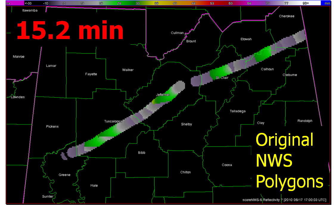
Average Departure Time (dt) = 15.2 minutes
Average False Time (ft) = 39.8 minutes
And recall the animation of the NWS warnings I provided in an earlier blog post:

What if we were to apply the Threats-In-Motion (TIM) technique to this event? Recall from this blog entry that I had developed a system that could automatically place the default WarnGen polygons at the locations of human-generated mesocyclone centroids starting at the same minute that the WFO issued its first Tornado Warning on the storm as it was entering Alabama. I used a re-warning interval of 60 minutes. If you adjust the re-warning interval to one minute (the same temporal resolution of the verification grids), you now have a polygon that moves with the threat, or TIM. The animation:

Let’s look at the verification numbers for the TIM warnings:
CSI = 0.2345
HSS = 0.3493
Average Lead Time (lt) = 51.2 minutes
Average Departure Time (dt) = 0.8 minutes
Average False Time (ft) = 23.1 minutes
Comparing the values between the NWS warnings and the TIM warnings visually on a bar graph:

All of these numbers point to a remarkable improvement using the Threats-In-Motion concept of translating the warning polygons with the storm, a truly storm-based warning paradigm. Let’s also take a look at how these values are distributed in several ways. First, let’s examine Lead Time. The average values for all grid points impacted by the tornado (plus the 5 km “splat”) are more than doubled for the TIM warnings. How are these values distributed on a histogram:


For the TIM polygons, there are a lot more values of Lead Time above 40 minutes. How do these compare geospatially?


Note that the sharp discontinuities of Lead Time (from nearly zero minutes to over 40 minutes) at the downstream edges of the NWS warnings (indicated by yellow arrows in the top figure) are virtually eliminated with the TIM warnings. You do see a few discontinuities with TIM; these small differences are caused by changes in the storm motions at those warned times.
Moving on to Departure Time, the average values for all grid points impacted by the tornado (plus the 5 km “splat”) are reduced to nearly zero for the TIM warnings. How are these values distributed on a histogram:


And geospatially:

With the TIM polygons, the departure times across the path length of both tornadoes is pretty much less than 3 minutes everywhere. Whereas, the NWS polygon Departure Times are much greater, and there are some areas still under the NWS warning more than 30 minutes after the threat had passed.
Finally, looking at False Alarm Time distributions both on histograms and geospatially:


There are some pretty large areas within the NWS polygons that are under false alarm for over 50 minutes at a time, even though these warnings verified “perfectly”. In comparison, the TIM warnings have a much smaller average false alarm times for areas outside the tornado path (about a 42% reduction). However, there are a number of grid points that are affected by the moving polygons for just a few minutes. How would we communicate a warning that is issued and then canceled just a few minutes later? That is food for future thought. I’ve also calculated an additional metric, the False Alarm Area (FAA), the number of grid points (1 km2) that were warned falsely. Comparing the two:
NWS FAA = 10,304 km2
TIM FAA = 8,103 km2
There is a 21% reduction in false alarm area with the TIM warnings, much less than the reduction in false alarm time. The reduction in false alarm area is more a function in the size of the warning polygons. The WarnGen defaults were used for our TIM polygons, but it appears that the NWS polygons were made a little larger than the defaults.
So, for this one spectacular long-tracked isolated supercell case, the TIM method shows tremendous improvement in many areas. But there are still some unanswered questions:
- How will we deal with storm clusters, mergers, splits, lines, etc.?
- How could TIM be implemented into the warning forecaster’s workload?
- How would the information from a “TIM” warning be communicated to users?
- How will we deal “edge” locations under warning for only a few minutes?
Future blog entries will tackle these.
Greg Stumpf, CIMMS and NWS/MDL
Precise Threat Area Identification and Tracking Part II: Threats-In-Motion (TIM)
Here I’m going to describe the “Threats-In-Motion”, or TIM concept that was presented at the 2011 National Weather Association Annual meeting. Essentially, once a digital warning grid is created using the methodology presented in the previous blog entry, the integrated swath product would start to translate automatically. The result would be that the leading edge of the polygon would inch downstream, and the trailing edge would automatically clear from areas behind the threat. We hypothesize that this would result in a larger average lead time for users downstream, which is desired. In addition, the departure time of the warning should approach zero, which is also considered ideal. The concept is first illustrated with a single isolated long-tracked storm for ease of understanding. Later, I will tackle how this will work with multi-cell storms, line storms, and storms in weak steering flow.
Why are Threats-In-Motion desired? Let’s look at the way most warning polygons are issued today. Threats that last longer than the duration of their first warning polygon will require a subsequent warning(s). Typically, the new warning polygon is issued as the current threat approaches the downstream end of its present polygon or when the present polygon is nearing expiration. This loop illustrates this effect on users at two locations, A and B. Note that only User A is covered by the first warning polygon (#1), even though its location is pretty close to User B’s location. Note too that User A gets a lot of lead time, about 45 minutes in this scenario. When the subsequent warning polygon (#2) is issued, User B is finally warned. However, User B’s lead time is only a few minutes, much less than User A who may only live a few miles away.

What if a storm changes direction or speed. how are the warnings handled today. Warning polygon areas can be updated via a Severe Weather Statement (SVS), in which new information is conveyed and the polygon might be re-shaped to reflect the updated threat area. This practice is typically used to remove areas from where the threat already passed, thus decreasing departure time. However, NWS protocol disallows the addition of new areas to already-existing warnings. So, if a threat areas moves out its original polygon area, the only recourse is to issue a new warning, sometimes before the original warning has expired. You can see that in this scenario:

Note that a 3rd polygon is probably required at the end of the above loop too!
In the past entry, I introduced the notion of initial and intermediate forecasted threat areas. The forecasted areas can update rapidly (one-minute intervals), and the integration of all the forecast areas results in the polygon swath that we are familiar with today’s warnings. But, there is now underlying (digital) data that can be used to provide additional specific information for users. I will treat these in later blogs:
- Meaningful time-of-arrival (TOA) and time-of-departure (TOD) information for each specific location downstream within the swath of the current threat.
- Using the current positions of the forecasted threat areas to compare to actual data at any time to support warning operations management
But what about “Threats-In-Motion” or TIM? Here goes…
Instead of issuing warning polygons piecemeal, one after another, which leads to inequitable lead and departure times for all locations downstream of the warning, we propose a methodology where the polygon continuously moves with the threat. Our scenario would now look like this:

Note that User A and User B get equitable lead time. Also note that the warning area is cleared out continuously behind the threat areas with time. And here is the TIM concept illustrated on the storm that right turned.

Now let’s test the hypotheses stated at the beginning of this entry. Does TIM improve the lead time and the departure time for all points downstream of the threat? If yes, what about the other verification scores introduced with the geospatial verification system, like POD, FAR, and CSI? The next blog entry will explore that.
Greg Stumpf, CIMMS and NWS/MDL