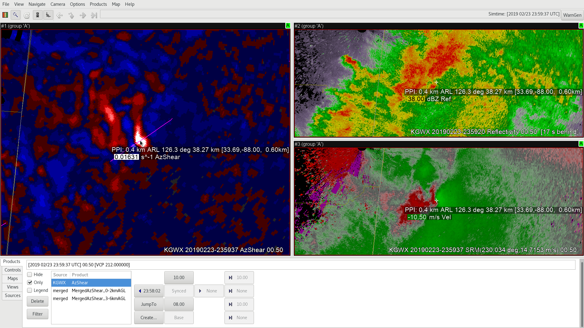
An example of AzShear for picking up on a weak circulation that later produced a short-lived tornado. This looks quite messy in reflectivity, with a weak circulation showing up on SRM. AzShear directs my attention here, and rightly so.

ZDR_Arcophile

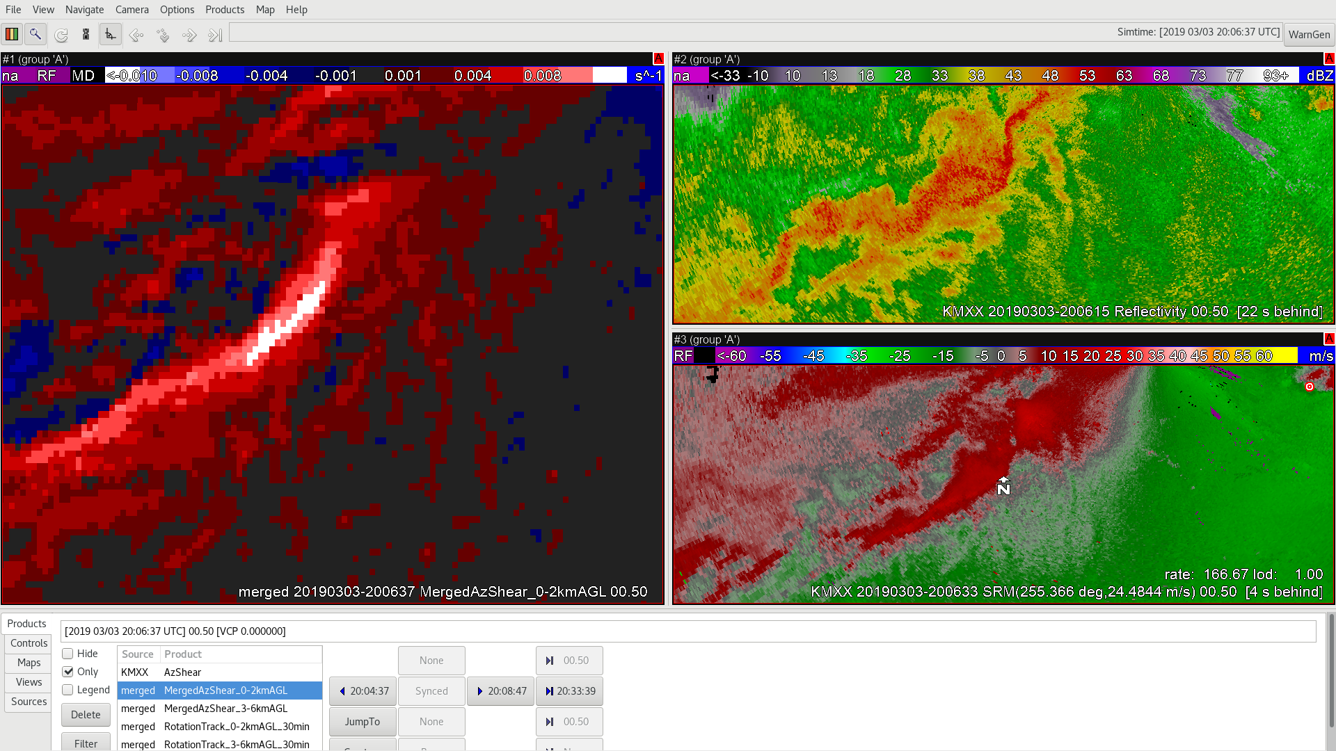
Very high utility here with the merged AZshear. Merged shear ramped up and after a couple of volume scans, My attention was drawn to an area that I would not have looked at by looking at SRM alone. This proved to be a developing tornadic situation over half an hour later! One caveat is that the area of circulation is not as precise as AzShear, of course.

ZDR_Arcophile

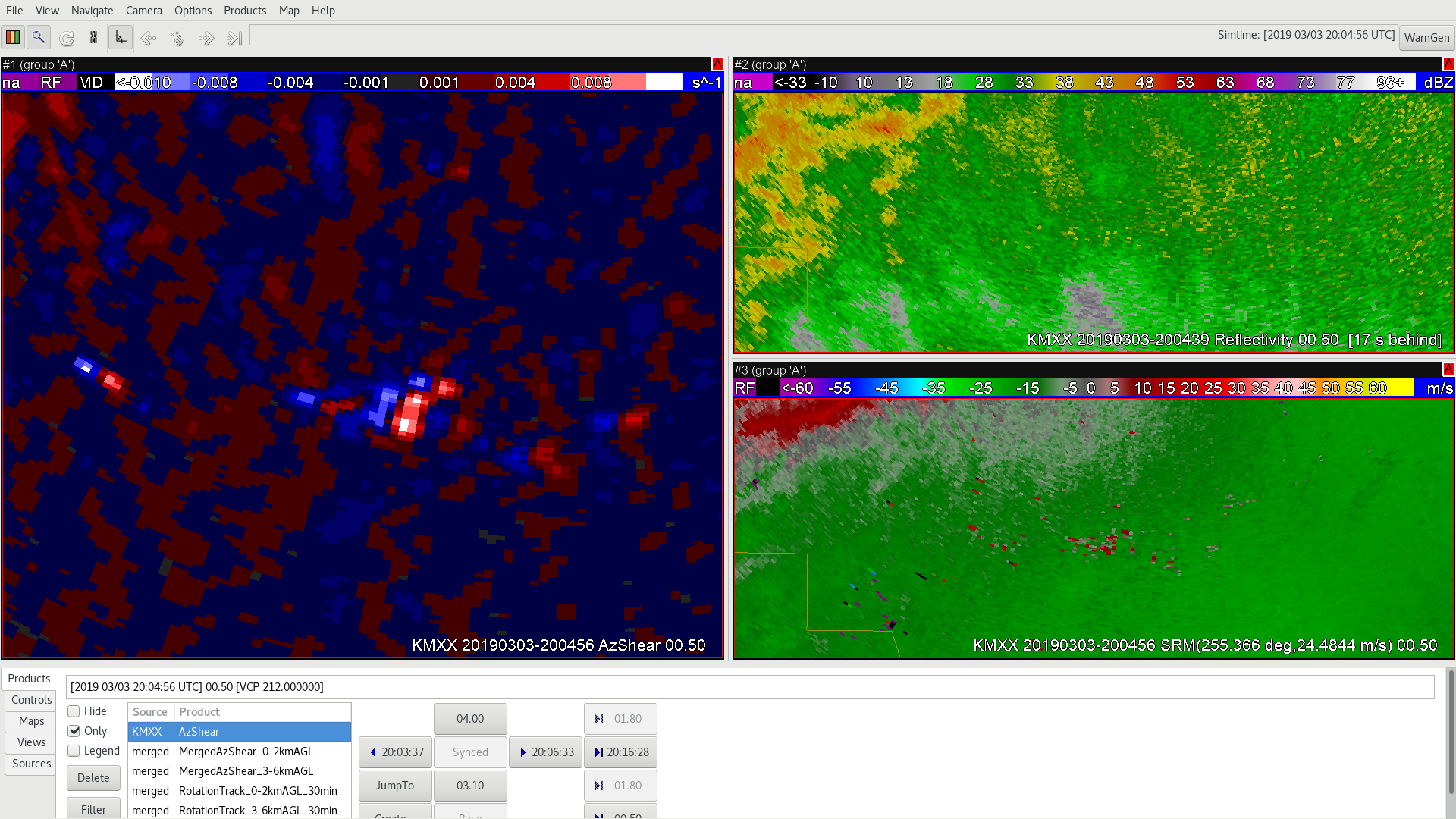
Here’s an example of where AzShear is VERY useful, especially if there are a lot of storms to look at. Here is a case where the AzShear is quickly ramping up and would alert me to a developing updraft well before I might catch this with SRM alone.

ZDR_Arcophile

AzShear can be noisy, but this can easily be recognized by viewing ref and SRM data concurrently.

ZDR_Arcophile

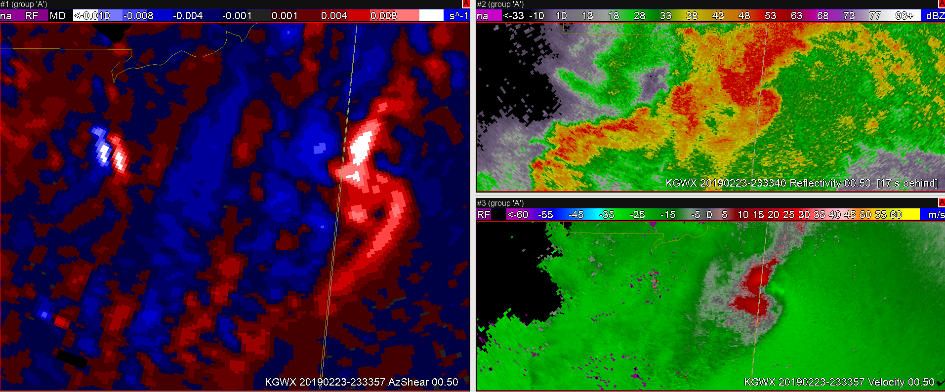
AzShear in this example, highlights the areas along the RFGF where vorticity is increasing, and eventually where the new tornadic circulation forms in several minutes. Something like this may be more identifiable in a radar looped image (especially with SRM), but in a still image a radar velocity scan may not be as intuitive.  In this instance, we see the AzShear output reduced after the previous tornado dissipates through occlusion…

But in the following image (at 2343 UTC) AzShear has already increased to ~0.015…

Tornadogenesis then occurs roughly 8 minutes later  (at 2351 UTC), with an AzShear value of ~0.016. Not much of an increase from the values 8 minutes earlier when GateToGate Shear was not present at the time.

Other thoughts…

• Long Term potential… Initial values of 1-D pseudo-vorticity is useful as base information, but values can mean different things at different elevations and distances from the radar. Would there be a way to eventually incorporate this information with AzShear for Climotological Tornadic Probabilities? Could help with ProbSVR model…
• Seems to handle noise relatively well, but certainly still shows waviness in the stable regions. Curious how this might preform in messier situations with surrounding precip. Merged AzShear handles much better than the base, but lag is a downfall.
• More experienced forecasters may use it well as initial checks, but oversimplification from a 1-D perspective may not translate as well to more inexperienced users. For example,  some less experienced users may equate the color white with a definite tornado, and non-white to no tornado. IDK… probably more of a communications issue unrelated to the product value.
• Would like to see how this performs in a more marginal case. for instance, some EF-0s within a QLCS.
• Has the potential to be a dangerous in areas of sidelobes! Perhaps a filter with Reflectivity may be helpful in these situations

#ProtectAndDissipate

The introduction to the single-site AzShear product as a broadcaster was exciting. The Mississippi case study was a good one to jump in with! Stepping through the data using AzShear, vel. and the refl data for the storm was very helpful. On most frames, the centroid of the AzShear maximum (or at least the visual maximum created through the colortable, with all values above 0.1 colored white), is right where I’d put the center of circulation using velocity.

This was confirmed when the observed tornado tracks from the survey were overlayed (purple) onto the data as seen in the image above from 2325Z.

A couple things jumped out to me in this analysis of this case study:

1. The AzShear values do drop a noticeable amount when the eastern Mississippi tornado lifts….which you’d expect both mathematically and conceptually given the gate to gate shear decrease as the velocity couplet deteriorates between 2329 and 2331Z after occlusion. (Note: tornado occurred with southern couplet – no tornado occurred with northern couplet strengthening between 2329 ans 2331Z)

2. In between the eastern Mississippi and western Alabama tornadoes, the AzShear values to return to +.01 and higher, prior to the second tornado occurring and velocity couplet signatures not looking as obvious as when the tornado is on the ground.

3. Is there value to seeing the data differences above .01? Colortable seems to indicate there isn’t, I’m sure published research exists regarding the importance of the values and the colortable choice.

-icafunnel

One unique advantage of the AzShear product I noticed (outside the initial 1-D vorticity analysis) was it’s ability to distinguish gust front boundaries very easily. In this example, you can easily distinguish the FFGF, the tornadic circulation, and the RFGF very quickly and can identify the supercell to be occluded with the RFGF pushing out away from the storm and is cutting off the low-level inflow into the storm. Sure enough, shortly after the supercellular circulation occludes, the tornadic circulation weakens and soon dissipates. In operations, this could be information easily identified by the forecaster noting the tornado may dissipate shortly.

#ProtectAndDissipate

This is a test blog for the Columbus, MS tornado on Feb 23, 2019

ZDR_Arcophile

AzShear has the potential to allow for sampling of the depth of rotation in any given storm in time and space to track the evolution of mesocyclones with time.  Before the surface circulation had developed, AzShear was starting to pick up on a strengthening mesocylone at approximately 3km.  Surface velocity products show weak cyclonic convergence starting to develop indicating that the potential was increasing for tornadogenesis sometime soon.  So, what did the time height look like?

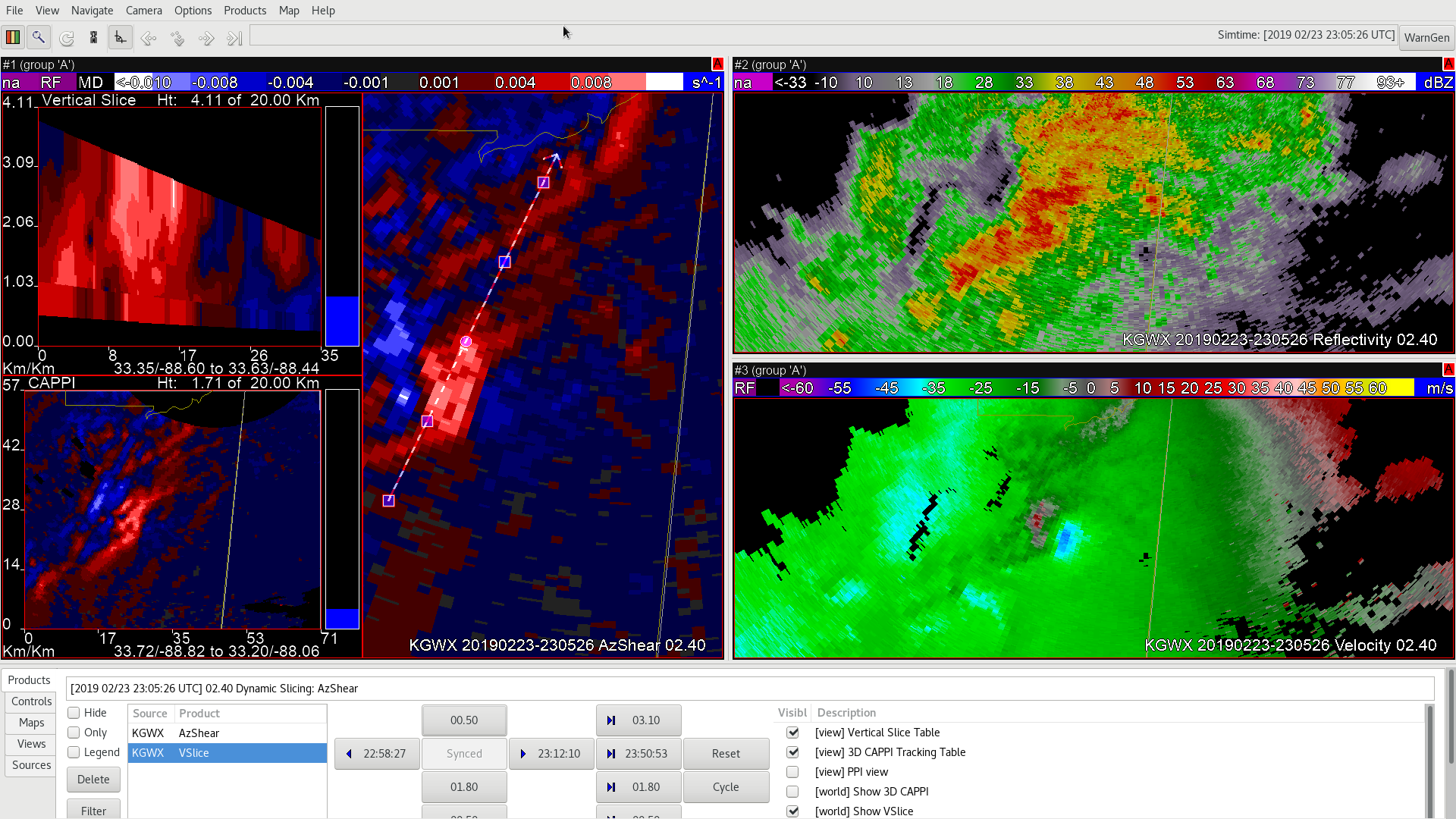
At 23:05:28, the strongest indications in AzShear were at the 2.4 degree tilt in this scan but were rather weak heading down to the lowest tilt (and there is an artifact in the cross section due to a time-matching issue with the SAILS scan).  Not shown is the descending positive AzShear values at or above 0.010 s^-1 with time so that by 23:11:34, the cyclonic shear had now reached the lowest scan:

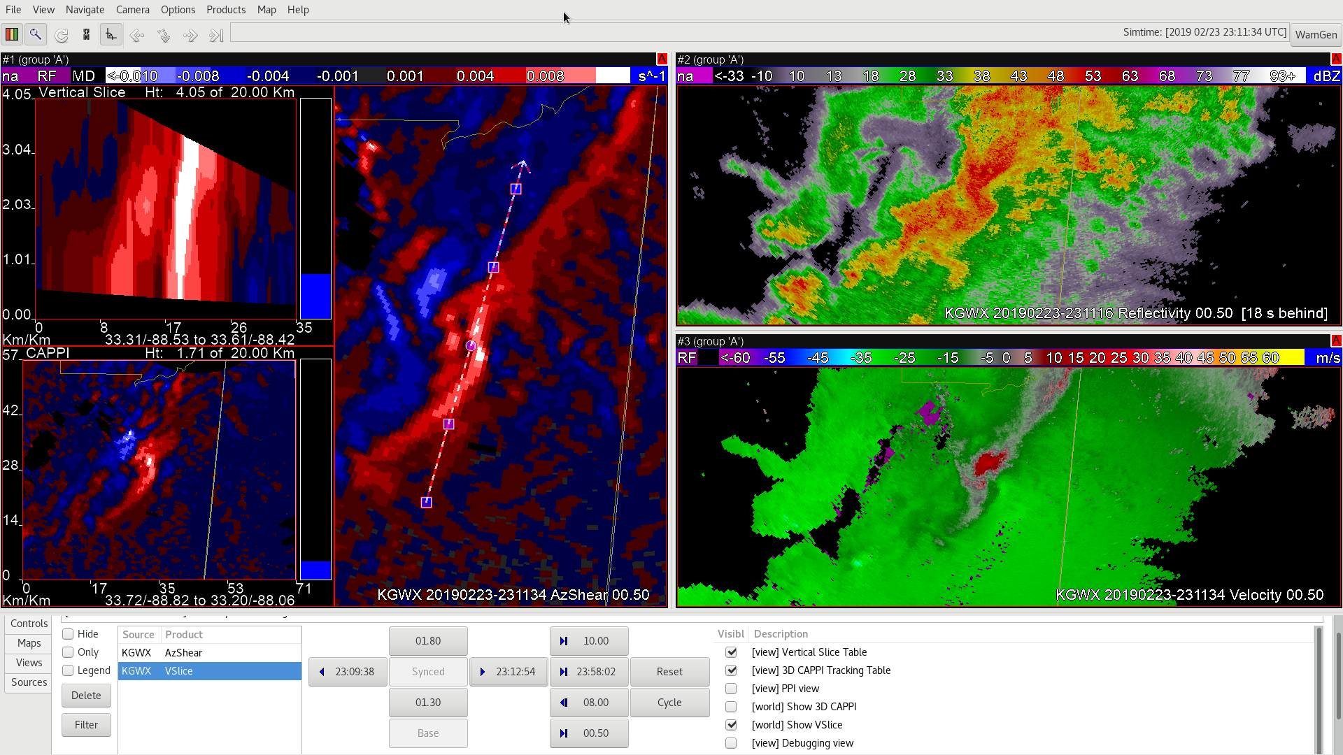
However, the lowest tilt shows that the tornado was possibly still in the process of forming as there was not a strong gate-to-gate couplet yet.  That took another 5 to 7 minutes depending on how strong of a couplet you want.  For this case, we’ll use 23:18:09: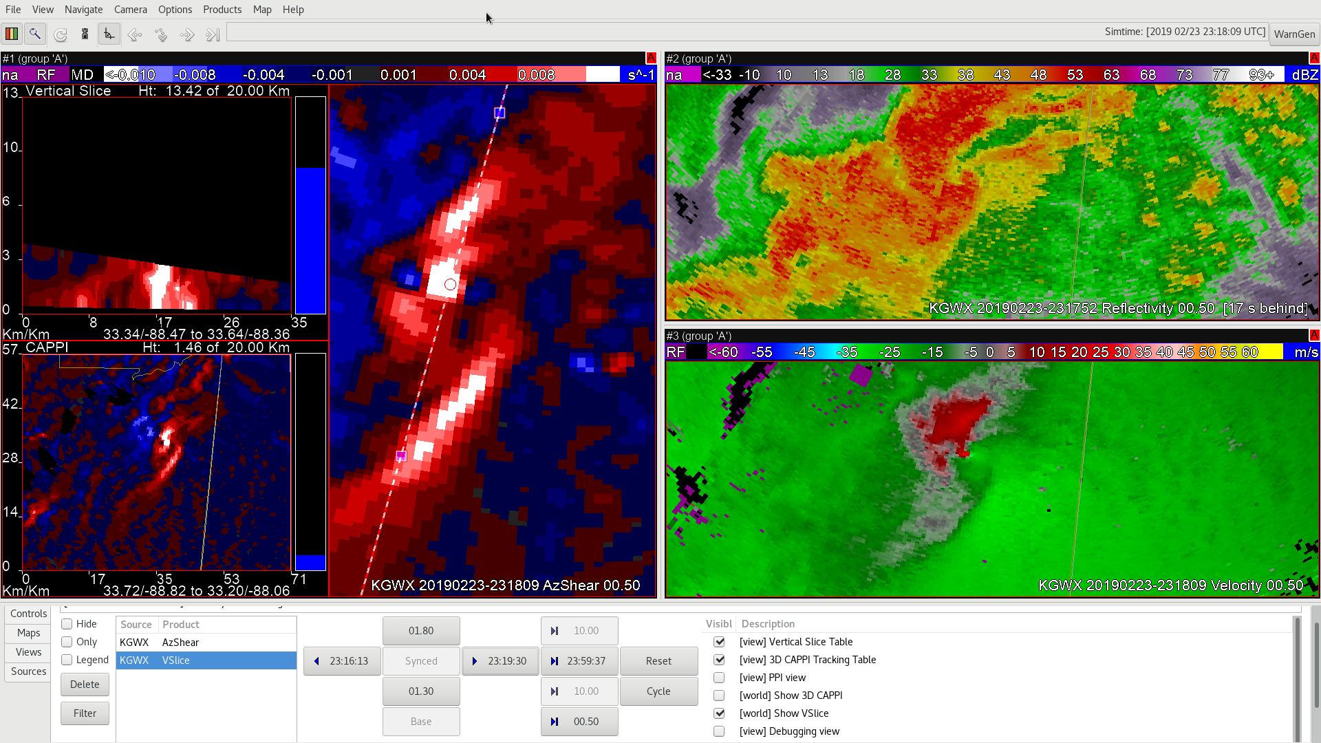

While the strong TVS remained intact, AzShear showed high positive values from the top of the cone of silence down to the lowest tilt.  Once the surface TVS and vortex appeared to have broken down, the mesocyclone aloft was still strong as shown in AzShear at 23:32:22:

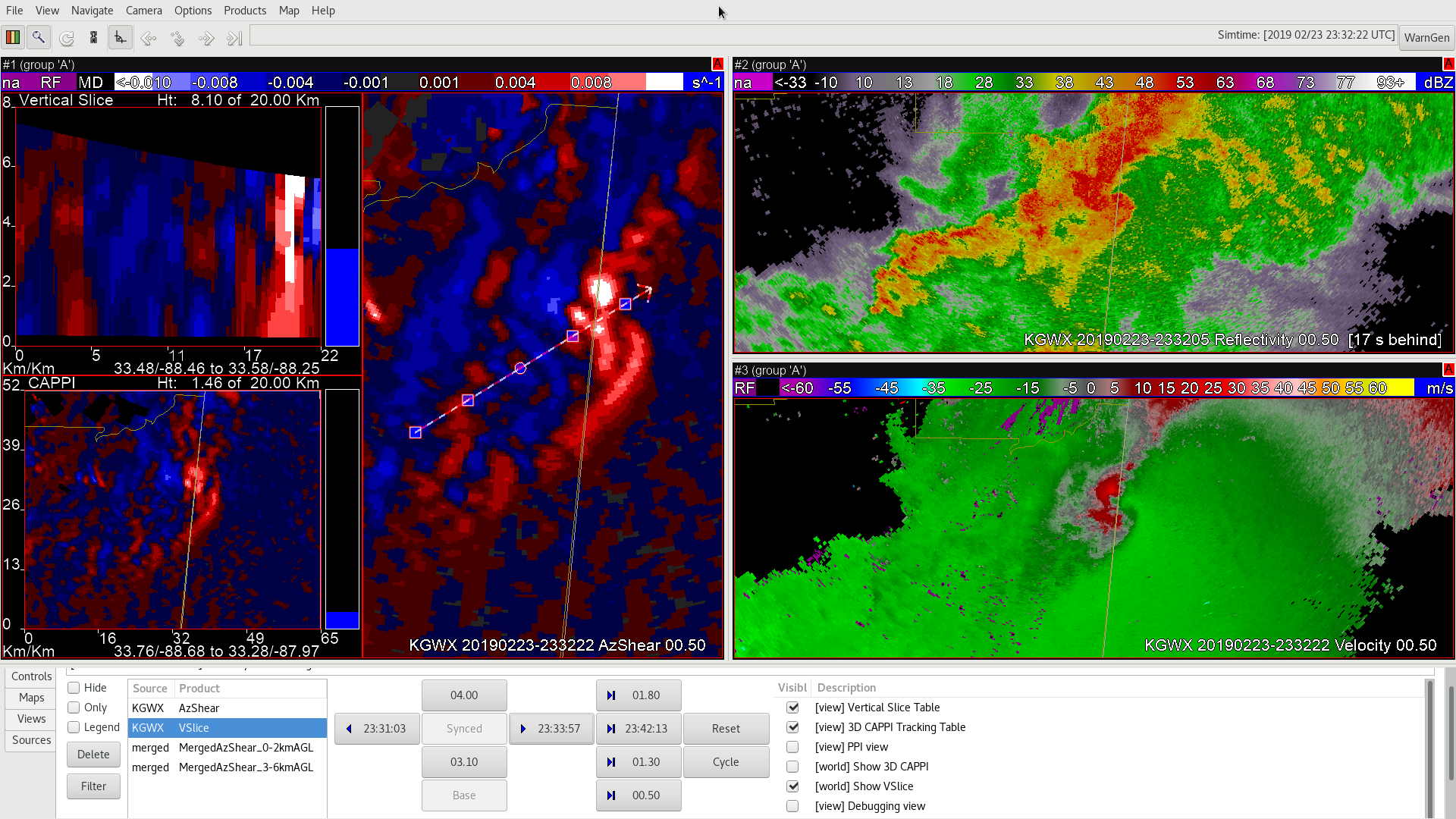
This indicates that there is utility in using AzShear in keeping situational awareness of what storms that are rotating are doing with time.  However, the usual caveats apply and YMMV:

1. Visualizing the 3-D structure using cross-sections will depend on how you place your cross section and how fast the storm is moving with time.  It may be impossible to do 2-D cross sections in 3-D space if the storm is moving fast!
2.  Since AWIPS doesn’t have 3-D rendering, the ability to accurately “paint” vertical circulations to see overall development is non-existent.
3. SAILS scans in WDSS-II (and potentially FSI) will not line up with the full Volume Scan so tracking of deep features will be limited at times, also complicating matters.

-Dusty

High positive & negative AzShear values were side by side in an area of drying/sinking air. Operational forecasters will need to keep an eye out for false high values and know when to discard that type of potentially misleading data. This is a good example of why it is still important to never focus on purely AzShear data in a warning environment.