A moderate risk of severe storms capable of producing large hail, damaging wind gusts and tornadoes occurred across the Dakotas. My focus was in the Bismarck, ND CWA where storms were likely initiating in eastern MT and then moving into the very unstable environment across western ND. All of the higher resolution models were a bit late on storm initiation as storms began to fire between 3-4 PM CT. The experiment began around 2 PM CT, which allowed for mesoanalysis of the pre-convective environment.

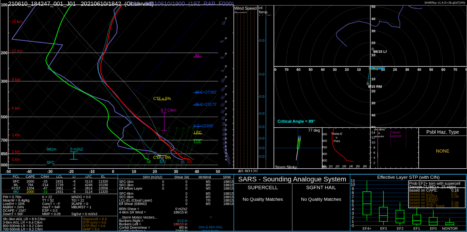
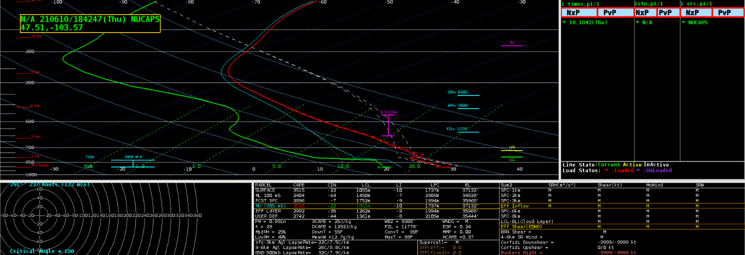
A NUCAPS CONUS NOAA-20 pass occurred at 19z across ND and then again at 20z where the eastern edge of this pass overlapped with the previous pass across western ND. At 19z, a comparison was made between the NUCAPS profile and a nearby RAP sounding at the same time. Below Image 1 shows the locations of the NUCAPS profile versus the RAP sounding. This area was chosen as it was close to where the satellite was showing some potential for convective initiation and was just east of the dryline in the area where the better instability was to be present.

Using sharppy the two profiles were then compared simultaneously. Both Images 2 and 3 show the two profiles, but image 2 will be highlighting the NUCAPS profile and associated instability values and image 3 will highlight the RAP sounding with associated instability parameters. Looking at the two profiles, there is not much difference in the mid to upper levels between the NUCAPS and RAP. However, the NUCAPS profile struggles more with the boundary layer features and temperature/dewpoint. Looking at observations, the current temperatures near that sounding location at 19z was 86 deg F with a dewpoint of 70 deg F. The RAP seemed to initialize these surface values pretty well and the thermodynamic profile east of the dryline, along with a bit of a capping inversion in place. Meanwhile, the NUCAPS profile struggled with the temperature and dewpoint, thus under doing the moisture and instability parameters. The CAPE values are noticeably different with the NUCAPS profile much lower with the instability due to these surface differences.

After seeing the discrepancies with the observed surface values versus the NUCAPS profile, I decided to grab the modified NUCAPS profile for the same location for comparison. Image 4 shows this modified sounding with a 10 degree difference between the non-modified surface temperature. The modified sounding shows a 82 deg F surface temperature, while the original NUCAPS profile had 91 deg F. With the cooler surface temperature the modified sounding showed a similar inversion to the RAP sounding between 750-800mb. The dewpoint temperature also was better representative of the actual surface dewpoint, which helped increase the instability parameters significantly. NUCAPS profiles tend to be a tad lower on the CAPE values, so the fact that the RAP is still about 1000 J/kg higher is not a surprise. However, with no RAOB sounding available and comparing the RAP with the modified NUCAPS profile there is quite a bit of similarity between the two in terms of the thermodynamic profile. Lastly, as storms begin to fire in the next hour or so and no RAOB profiles closeby, it might be useful to compare and utilize the temperature heights (0, -10, -20, and -30 deg C) for radar interrogation as storms initiate. Knowing the RAP and modified NUCAPS profiles were similar then the heights from the temperature levels could also be compared. The RAP does show higher heights than the modified NUCAPS profile, so this is something to keep in mind and monitor as storms fire along the dryline.

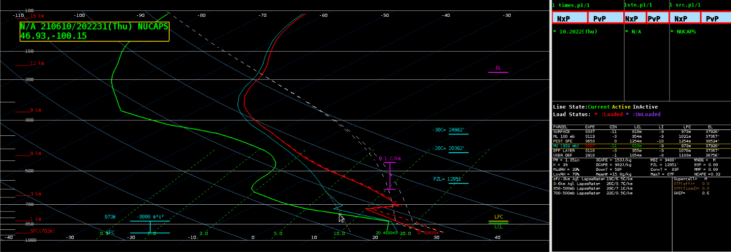
Keeping with the theme of NUCAPS, there was another pass at 20z further west (as mentioned at the beginning) that overlapped the 19z pass in parts of western ND. This included the town of Bismarck, where the office put out a special 20z RAOB sounding. Bismarck was a bit further east than the previous sounding, but was still in the very favorable environment. Images 5 and 6 show the comparison between the NUCAPS sounding at 20z and the RAOB Bismarck special sounding at the same time. Similar results can be seen between the observed sounding and NUCAPS profile where the CAPE values are again lower in the satellite derived sounding. This time the NUCAPS profile did a much better job with the surface temperature and despite the temperature profile being a bit smoother due to lack of detail in the boundary layer, the profile was overall pretty similar to the RAOB temperature profile. The dewpoint profile on the NUCAPS was much drier at the surface and therefore had a bit of a drier boundary layer than the observed sounding, which is likely why the CAPE values are also a bit lower.

Once again the modified NUCAPS profile was compared (Image 7 below). The modified profile did a better job at showing the moisture in the boundary layer and attempted to pick up the dry layer at 650mb, which was actually at 700mb on the RAOB profile. Unfortunately, the temperature was too low and therefore the modified NUCAPS temperature profile shows a very sharp capping inversion that was unrealistic. Overall, the CAPE values did increase with the modified sounding versus the original NUCAPS profile and were closer to the observed sounding. Twice it has been noted that the heights of the temperature levels were closer between the non-modified NUCAPS profiles with the model/observed soundings. There may be some calculation in the modified sounding that is causing the heights to be lower and maybe unrealistic. In scenarios where there is a RAOB sounding, that is the best picture of the atmosphere you can get but it is great to compare the NUCAPS profiles for comparison to future events and potential trends in the satellite derived soundings.

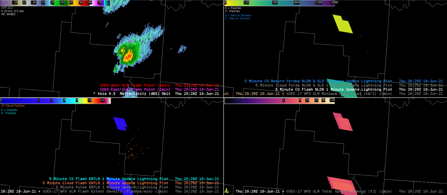
As storms began to initiate across eastern MT, both G16 and G17 GLM were utilized to look for lightning instances in the growing storms. Having both satellites can be super helpful, especially when one viewing angle may not see the strike, while the other does. This happened several times during storm initiation where one satellite would pick up a strike, while the other displayed nothing. Images 8-9 show this occurring twice in two different storms where each satellite picked up a strike that the other did not. As mentioned before, the viewing angle may not be in a good position for the satellite to see the storm’s top and therefore the strike is not bright enough to be detected. Along those lines, the scattering properties in the cloud are also not visible by the angle of the satellite’s view point and could cause the satellite to miss a strike. Lastly, there is a quality assurance that occurs for each product and if the strike wasn’t strong or long enough then the pixel could have been tossed out during this quality assurance. This is why it is so important to utilize both satellites when possible and it is a best practice to err on the side of whichever satellite is showing more lightning is probably more accurate.

ProbSevere version 2 and 3 were compared through the afternoon. The trend continued with version 2 remaining about 20-30% higher in all categories except the tornado probs. Version 3 has leaned towards being slightly higher than version 2 when it comes to tornado probabilities. ProbSevere time series was utilized to track the southernmost storm along the line of storms headed into western ND during the mid afternoon hours. Both radars were pretty far away on either side of the storms, with Glasgow’s radar being slightly closer. The lowest elevation scan was at around 13000-14000 feet when velocity began showing a strong mesocyclone. Image 10 shows the time series of ProbSevere and the readout comparing version 3 with version 2. All four ProbSevere categories were steadily increasing through the last hour with version 2 remaining higher than version 3. Version 2 shows close to 100% probabilities for all but tornado, making this storm look like a slam dunk due to the environmental parameters.  Meanwhile version 3 is slightly lower due to the fact that it can pick up on similar storms that occurred in a similar environment with little to no reports (from storm data). This is where version 3 adds in a bit more information to create more realistic probabilities.

Based on the strong rotation in Image 10, the tornado probabilities were close to 30 percent which is relatively high and should give a forecaster confidence on issuance with a lack of lower level radar scans. Chaser footage also helped to back the need for a tornado warning with images of wall clouds, funnels and more being reported from multiple sources. Image 11 shows the time series for ProbSevere along with multiple other parameters. One thing that was interesting to see was the tornado probability drastically dropped in version 2 but remained steady in version 3. Since version 2 is heavily using az shear, you can see the drop in MRMS az shear (red line on second plot down on the far left), which could be correlated with that probability drop in version 2. Also, the MLCIN is slowly increasing (blue line on second plot down on the far right) and could be playing a bit of a role in this drop as well. This is where version 3 might have a leg up on version 2 when it comes to tornado probabilities.

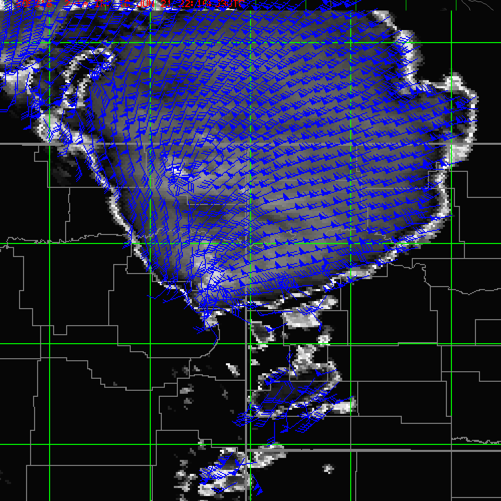
Lastly, the optical winds were utilized to see the winds at the top of the storm. Image 12 shows the optical wind field for 200-100mb. You can see the cooler cloud tops in satellite below the wind field and then the associated diffluence aloft. This is an indication of the very strong supercell that is showing no signs of weakening anytime soon. Also, it is of note that there is another cool cloud top signature a bit further to the northwest associated with another strong supercell with diffluence aloft. The optical wind fields are useful in knowing what is going on aloft and the potential strengthening or even weakening of a storm.

– Harry Potter