AzShear in Situational Awareness

Here’s an example of where AzShear is VERY useful, especially if there are a lot of storms to look at. Here is a case where the AzShear is quickly ramping up and would alert me to a developing updraft well before I might catch this with SRM alone.

ZDR_Arcophile

AzShear – Increasing Vorticity Along RFGF

AzShear in this example, highlights the areas along the RFGF where vorticity is increasing, and eventually where the new tornadic circulation forms in several minutes. Something like this may be more identifiable in a radar looped image (especially with SRM), but in a still image a radar velocity scan may not be as intuitive.  In this instance, we see the AzShear output reduced after the previous tornado dissipates through occlusion…

But in the following image (at 2343 UTC) AzShear has already increased to ~0.015…

Tornadogenesis then occurs roughly 8 minutes later  (at 2351 UTC), with an AzShear value of ~0.016. Not much of an increase from the values 8 minutes earlier when GateToGate Shear was not present at the time.

Other thoughts…

  • Long Term potential… Initial values of 1-D pseudo-vorticity is useful as base information, but values can mean different things at different elevations and distances from the radar. Would there be a way to eventually incorporate this information with AzShear for Climotological Tornadic Probabilities? Could help with ProbSVR model…
  • Seems to handle noise relatively well, but certainly still shows waviness in the stable regions. Curious how this might preform in messier situations with surrounding precip. Merged AzShear handles much better than the base, but lag is a downfall.
  • More experienced forecasters may use it well as initial checks, but oversimplification from a 1-D perspective may not translate as well to more inexperienced users. For example,  some less experienced users may equate the color white with a definite tornado, and non-white to no tornado. IDK… probably more of a communications issue unrelated to the product value.
  • Would like to see how this performs in a more marginal case. for instance, some EF-0s within a QLCS.
  • Has the potential to be a dangerous in areas of sidelobes! Perhaps a filter with Reflectivity may be helpful in these situations


#ProtectAndDissipate

AzShear Introduction – Feb 23 Case Study

The introduction to the single-site AzShear product as a broadcaster was exciting. The Mississippi case study was a good one to jump in with! Stepping through the data using AzShear, vel. and the refl data for the storm was very helpful. On most frames, the centroid of the AzShear maximum (or at least the visual maximum created through the colortable, with all values above 0.1 colored white), is right where I’d put the center of circulation using velocity.

This was confirmed when the observed tornado tracks from the survey were overlayed (purple) onto the data as seen in the image above from 2325Z.

A couple things jumped out to me in this analysis of this case study:

  1. The AzShear values do drop a noticeable amount when the eastern Mississippi tornado lifts….which you’d expect both mathematically and conceptually given the gate to gate shear decrease as the velocity couplet deteriorates between 2329 and 2331Z after occlusion. (Note: tornado occurred with southern couplet – no tornado occurred with northern couplet strengthening between 2329 ans 2331Z)


2. In between the eastern Mississippi and western Alabama tornadoes, the AzShear values to return to +.01 and higher, prior to the second tornado occurring and velocity couplet signatures not looking as obvious as when the tornado is on the ground.

3. Is there value to seeing the data differences above .01? Colortable seems to indicate there isn’t, I’m sure published research exists regarding the importance of the values and the colortable choice.

-icafunnel

AzShear RFGF – Occluded Supercell

One unique advantage of the AzShear product I noticed (outside the initial 1-D vorticity analysis) was it’s ability to distinguish gust front boundaries very easily. In this example, you can easily distinguish the FFGF, the tornadic circulation, and the RFGF very quickly and can identify the supercell to be occluded with the RFGF pushing out away from the storm and is cutting off the low-level inflow into the storm. Sure enough, shortly after the supercellular circulation occludes, the tornadic circulation weakens and soon dissipates. In operations, this could be information easily identified by the forecaster noting the tornado may dissipate shortly.

#ProtectAndDissipate

CPTI example

CPTI closely followed the 0-2 Az Shear product in both shape and intensity. This included all velocity time matching errors. These time matching errors decreased the usefulness of the product each time they were seen. CPTI prob of highest winds appeared more useful than the lower thresholds, better enhancing where the threat of strong winds was actually located. Lower thresholds (example at end of loop) appeared to be too broadbrushed for applicable use.

Odd AzShear data: 22:16

Az shear shows a double scan signature on the top left here. This seems like it would result from SGF scanning the shear at one time and Tulsa hitting it at another. Clearly there are not two lines of shear here per radar single scans.

Another example of a double AzShear signal. Likely coming from radar timestamp matching issues.

Tags: None

HWT day 2: 19:10 GLM and AzShear observations of Missouri tornadic supercell

Feature following zoom showing the GLM pulsing phenomena associated with intensification/weakening of a supercell in OK/MO. During the third pulse, a TOR warning was issued.

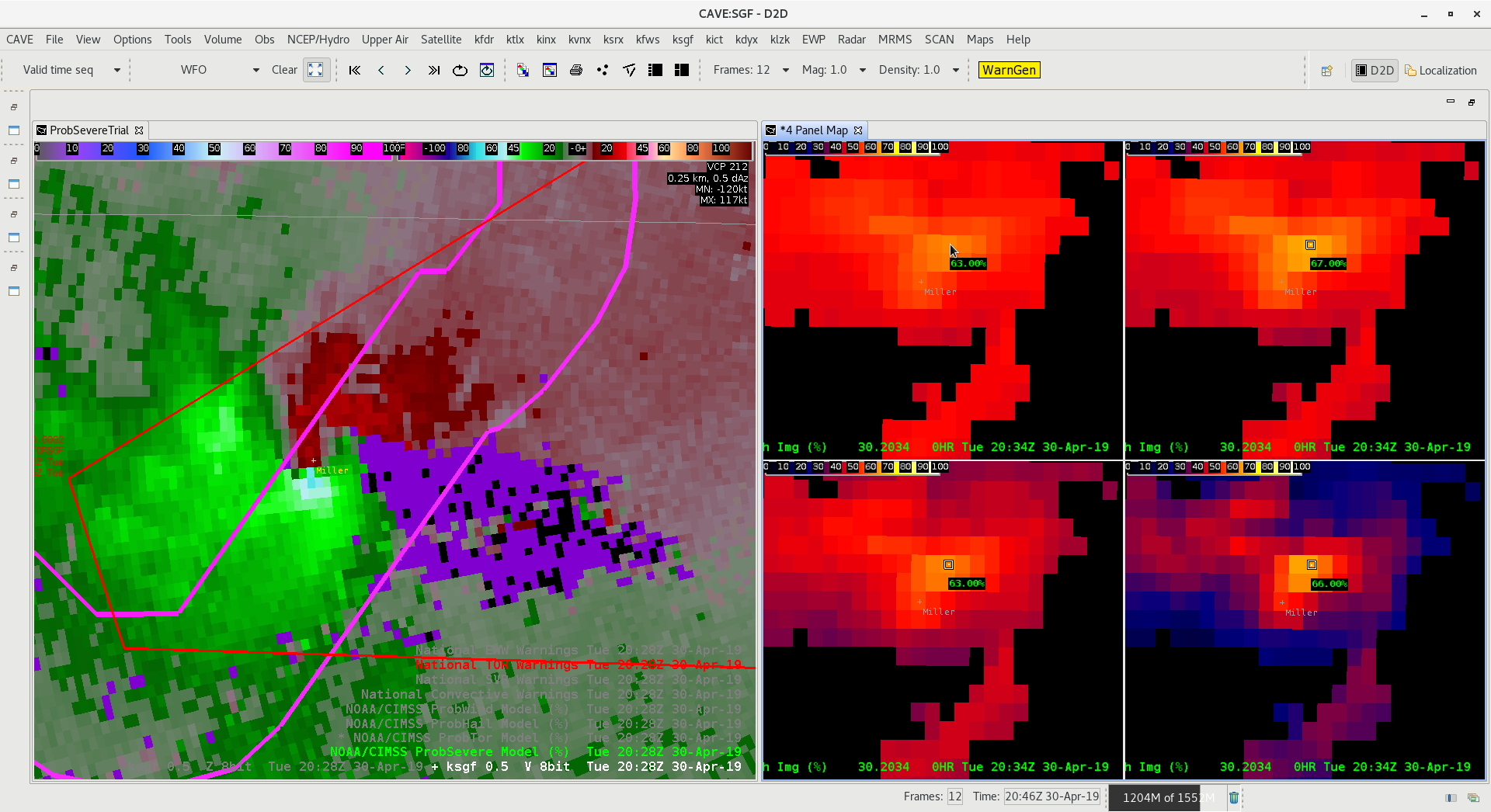
Case of CPTI values on a confirmed tornado near Miller, MO. No confirmed damage estimates yet, but TOR was confirmed at this time visually and with a TDS

Lightning jump preceding a tornado and then confirmed touchdown in MOEvent Density over the same cell

Minimum Flash area showing updraft core


Average Flash Area


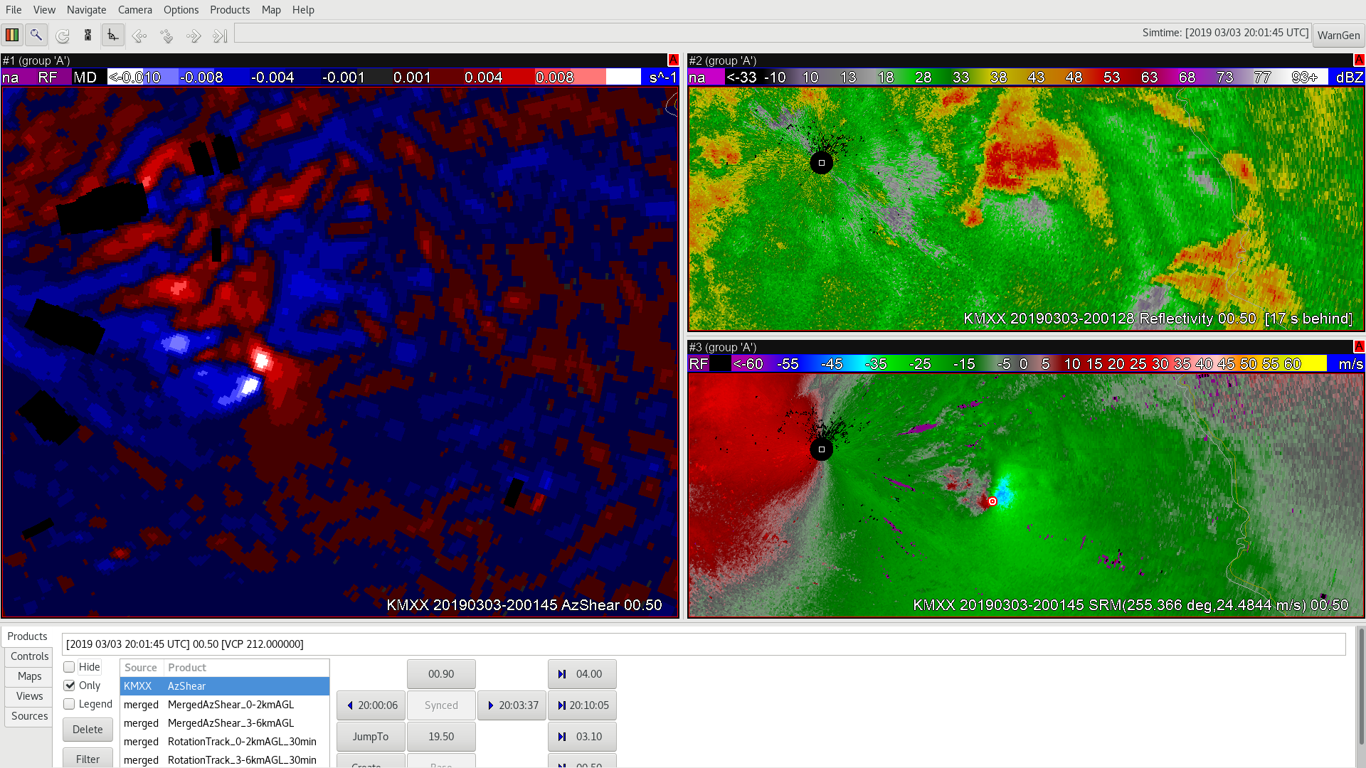
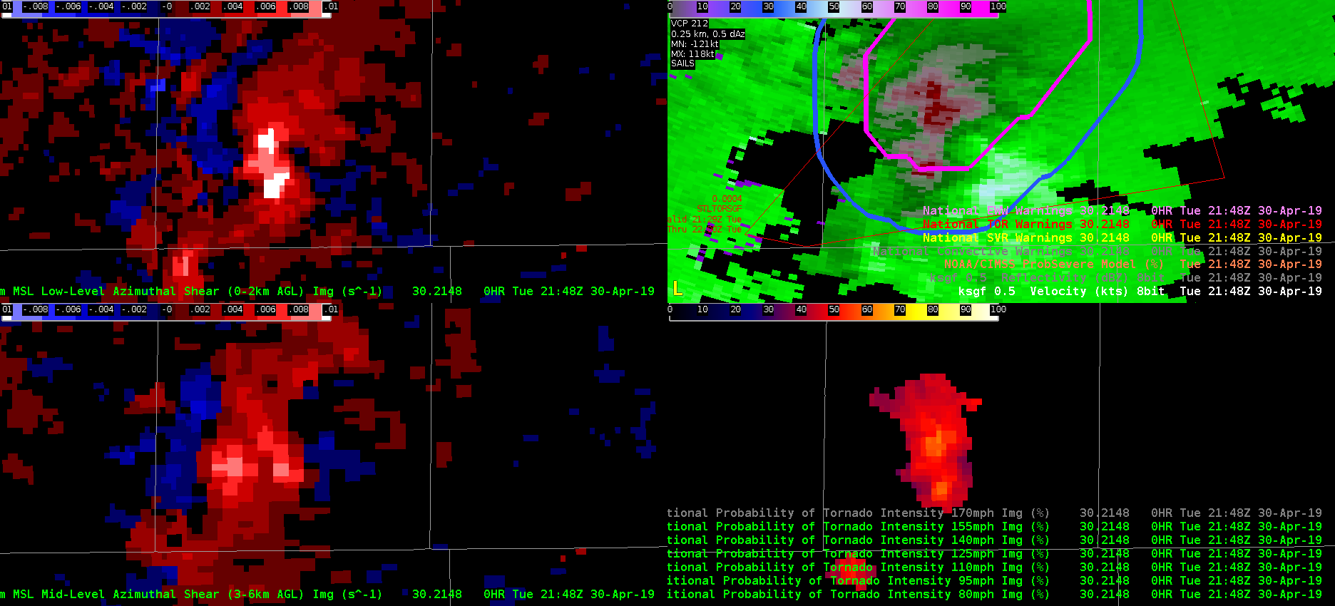
This is a case where AzShear overdid the tornadic threat This supercell had a circulation that never really tightened up. ProbSevere also vastly overestimated the tornado threat, likely due to nearby storm interactions and mergers. When convection gets messy, can we rely on these products as much?


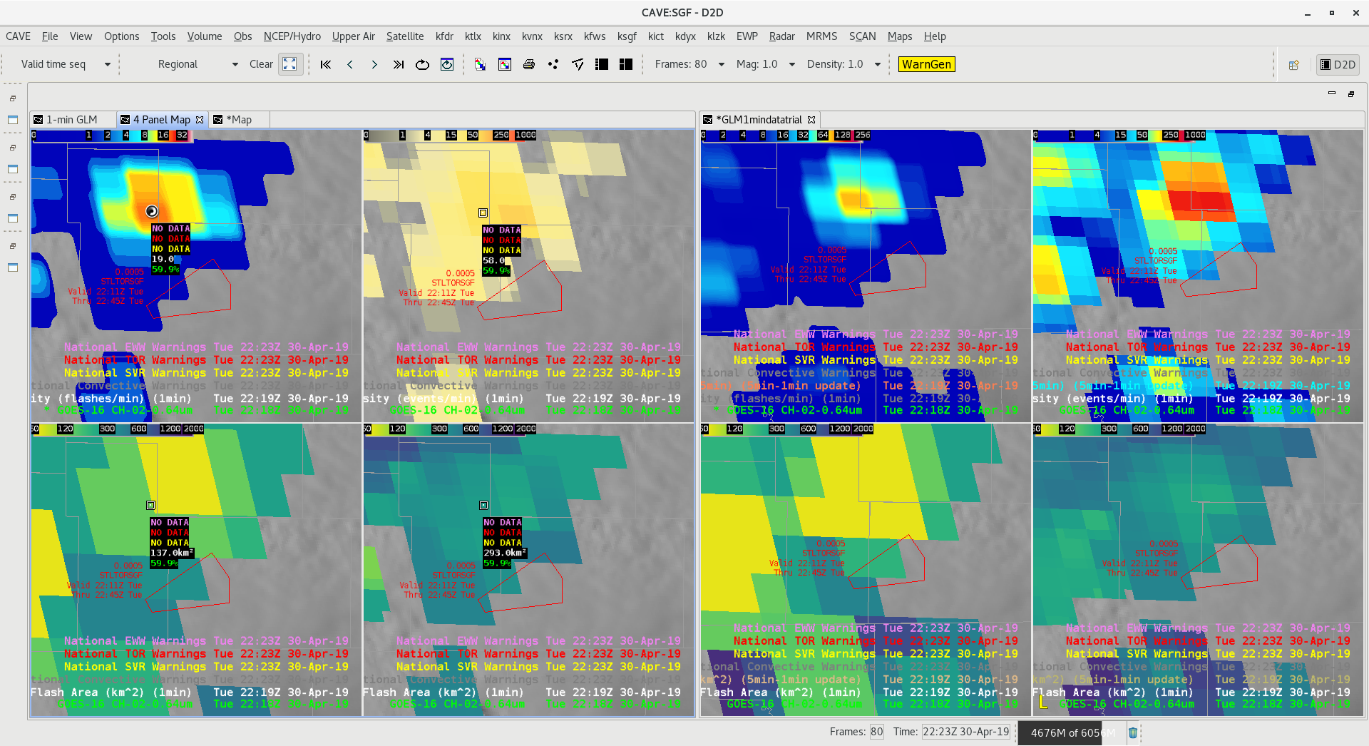
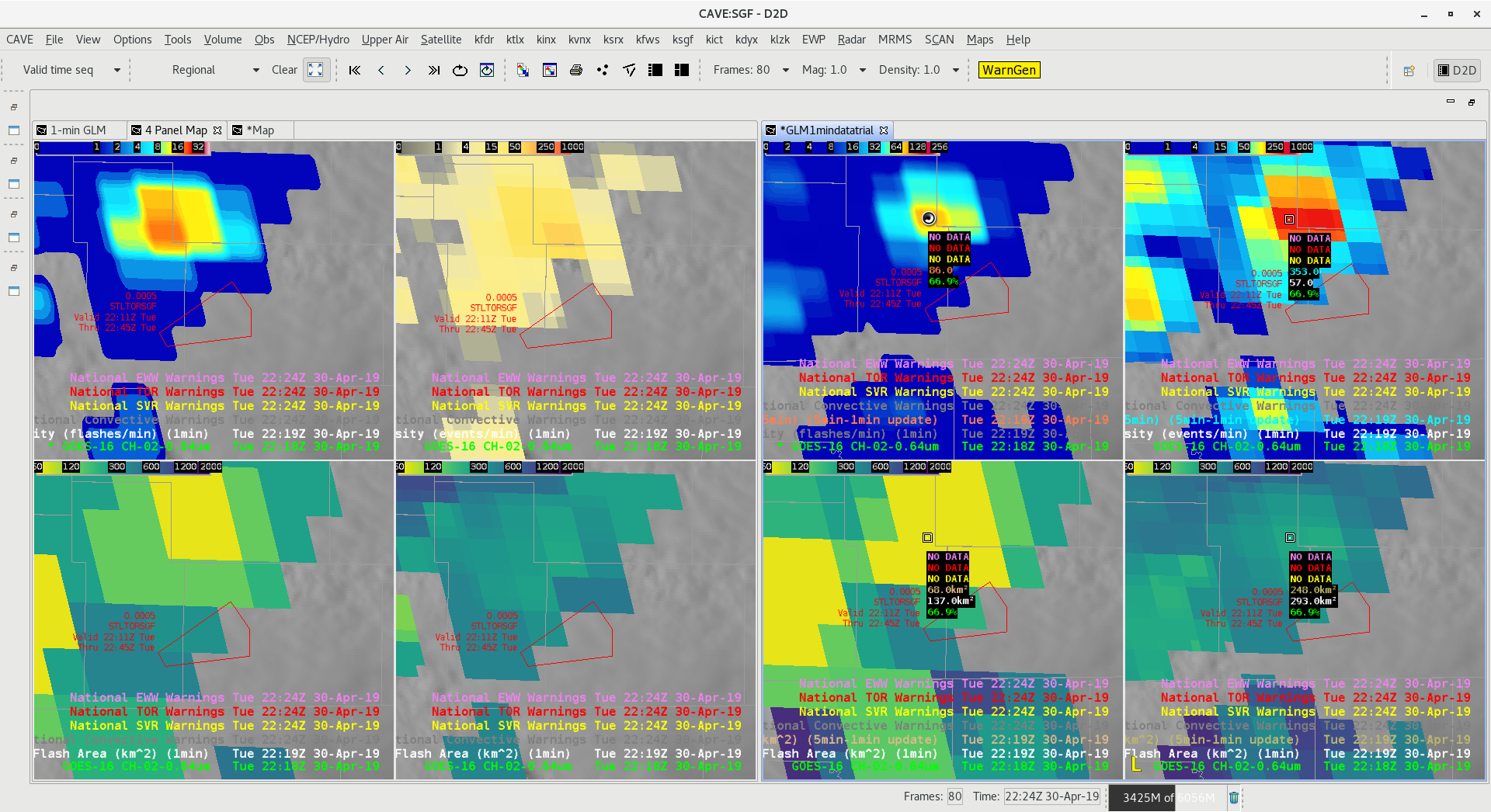
The two images above compare a 4 panel of 1 min GLM data (left four panels) versus 5 min data (right four panels). While the 5 min data was much smoother to view from an animation and trend sense, the 1 min data did provide some fine temporal resolution help during periods of rapid storm intensification preceding this tornado warning.

The above two loops compare 1 min looping (top 4 panel) versus 5 min looping (bottom 4 panels). In a loop the ‘flashy’ nature of 1 min data makes it less desirable in operations, however manual toggling and advancing still make this data useful.
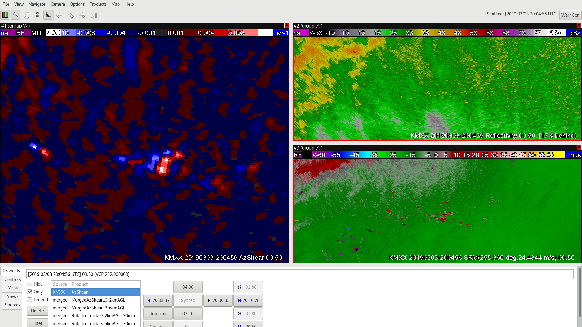
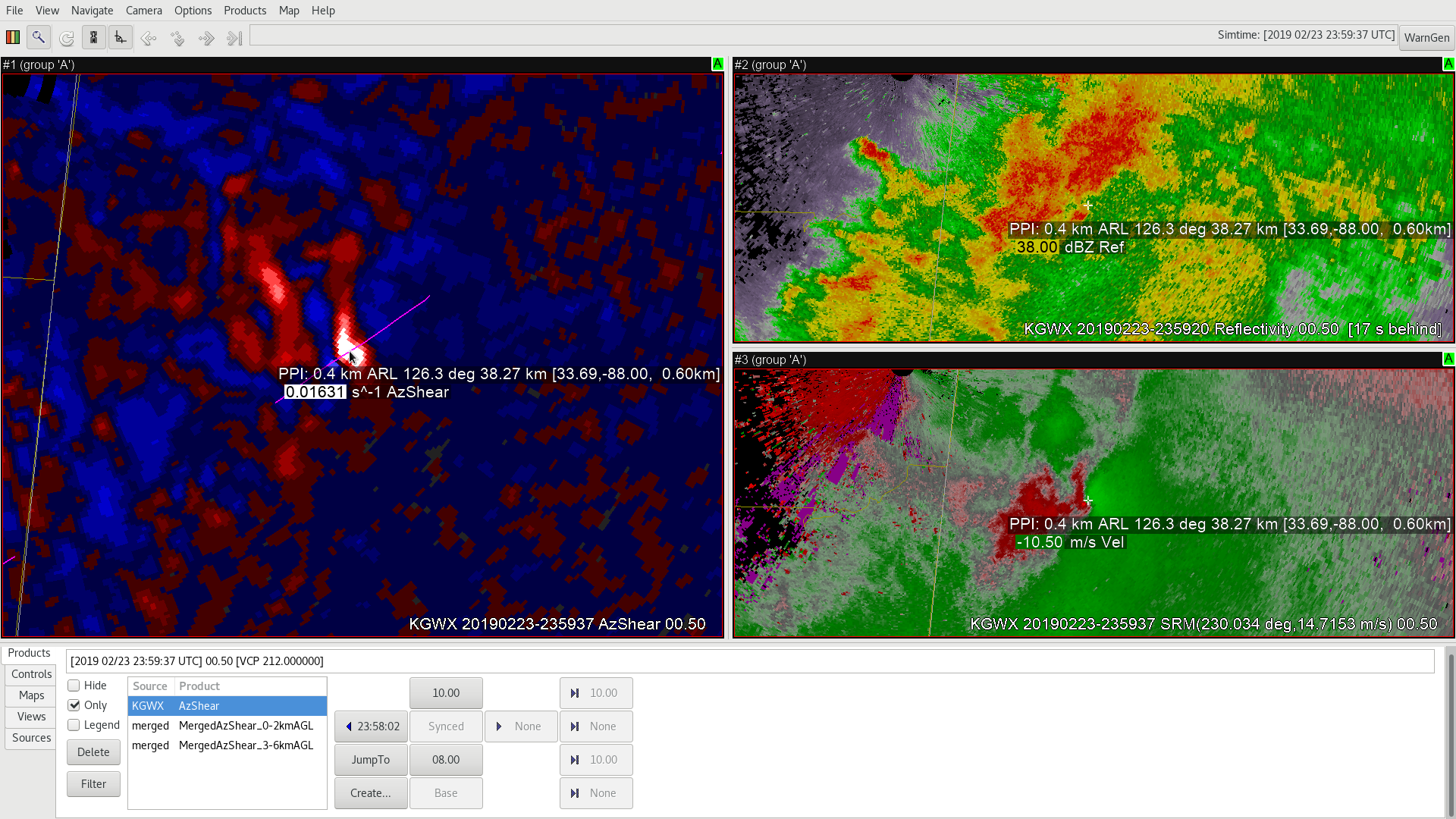