The forecast experiment centered on ABI (Abilene, TX) today to catch development along the dryline and other moisture gradients, including a warm front eroding the morning’s stratus northward. After analyzing and discussing the 12Z sounding plan views, we had about an hour on the schedule to create the 20-00 UTC and 00-04 UTC forecasts. It turns out we took a bit more than 90 minutes, since there were three scenarios we considered: (a) Convective initiation over the mountainous terrain of southwest Texas, coverage, and mode as forcing moved east; (b) Same initiation, coverage, and mode problem but over the South Plains and panhandle of Texas and extreme southwest Oklahoma, and; (c) what to think about some model members’ convection forecasts over southeastern Texas.

The forecast team I participated in wrestled with forcing mechanisms since the shear profiles were less than robust over the central and southern portions of west Texas and looked to be favorable in the panhandle, South Plains, and extreme southwest Oklahoma. We (there were six of us on the team today) settled on two initiation scenarios–the first in southwest Texas in the 20-21 UTC time frame as a shortwave moved toward El Paso and a second toward the space of Texas between Amarillo and Lubbock with a second jet streak moving into the area. The third area was discounted based on standard theories of organized severe convection.

For ensemble displays, we used

1. The probability of 40 dBZ reflectivities. This helped focus our attention on the areas of concern and timing scenarios. This is probably the quickest way to assess the result of each model’s integration rather than interrogating multiple plan views, soundings, and postage stamp images of significant fields.
2. Spaghetti outlines of 40 dBZ model-derived reflectivity. This is a noisy but useful depiction.
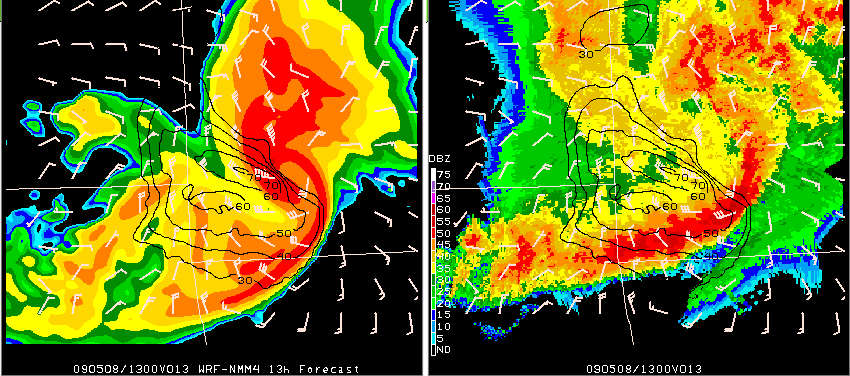
3. Max reflectivity from the ensemble members to assess in a very rough manner storm instensity, and
4. Max updraft helicity to assess the likelihood of severe weather.

From these we went to individual high-res (1-4 km) models and the observations to modify the threat area. It’s interesting to note that most participants prefer to use a single high-res or a familiar lower-res (e.g., 12 km WRF-NMM) as assess potential mode and than use the ensembles to place mental “possibilities” around what I’d call the “individual’s most probable” forecast.

The deterministic and ensemble runs suggested that southern storms would like be isolated and probably end short after 01 UTC. In the north we believed more organized convection, possibly a couple of clusters, was likely due to the presence of better 0-6 km shear. The was some issue as to how far east the convection would progress by 04 UTC, with the 1 km models suggesting propagation as far east as I-35. The operational SPC forecaster acting as our team’s guide tempered our enthusiasm with a little climatology, so the east edge of our forecast area was kept a little west (upstream) of the most aggressive model’s 04 UTC position for convection.

We believed there was a significant hail threat over this area given the shear, mid-level lapse rates, and NAM-KF model soundings suggesting analogs of 2+” hail cases. SPC’s significant hail paramenter on its mesoanalysis page also centered a threat in this area.

As I write this, we were not far enough west with our initiation and the severe threat is continuing a bit north of the area we anticipated. Tomorrow’s review ought to be quite enlightening, assuming we can keep our brains focused on the review and not on Wednesday’s expected event!

— Bruce E, forecasting on the West team today