
I am posting late this week. It has been a wild ride in the HWT. The convection initiation desk has been active and Tuesday was no exception. The threat for a tornado outbreak was clear. The questions we faced for forecasting the initiation of storms were:
1. What time would the first storms form?
2. Where would they be?
3. How many episodes would there be?
This last question requires a little explanation. We always struggle with the criteria that denotes convection initiation. Likewise we struggle with how to define the multiple areas and multiple times at which deep moist convection initiates. This type of problem is “eliminated” when you issue a product for a long enough time period. Take the convective outlook for example. Since the risk is defined for the entire convective day you can account for the uncertainty in time by drawing a larger risk area and subsequently refining it. But as you narrow down your time window (from 1 day to 3 hours or even 1 hour) the problems can become significant.
In our case, the issue for the day was compounded because the dryline placement in the models was significantly east of the observed position by the time we started making our forecast. We attempted to account for this fact and as such had to adopt to a feature relative perspective of CI along the dryline. However, the mental picture you are assembling of the CI process (location, timing, number of episodes, number of storms) is tied not just to the boundaries you are considering, but the presumed environment in which they will form.
The feature relative environment then would necessarily be in error because we simply do not have enough observations to account for the model error. We did realize that shallow moisture, which was shown on morning soundings, was not going to be the environment in which our storms formed. Surface dew points were higher and staying near 68 in the warm sector. We later confirmed this with soundings at LMN which showed the moist layer increase in depth with time.
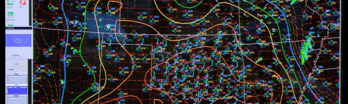
So we knew we had two areas of initial storm formation, one in the panhandle of OK and into KS along the cold front to the west and triple point to the east. The other area was along the dryline in OK and TX. We had to decide how far south storms would initiate. As we figuring all of this out, we had to look at the current satellite imagery since that was the only tool which was accounting for the correct dryline placement and estimate how far east it might travel, or mix out to in order to make the forecast.
Sure enough, the warm sector had multiple cloud streets ahead of the dryline. Our 4km model suite is not really capable of resolving cloud streets but we still needed to make our forecast roughly 1-2 hours before CI. So in a sense we were not making a forecast as much as we were making a longer more uncertain nowcast (probably not abnormal given the inherent unpredictability of warm season convection). Most people put the first storm in KS and would end up being quite accurate in placement. Some of us went ahead of the dryline in west central OK and were also correct.
There was one more episode in southern OK and then another in TX later on. This case will require some careful analysis to verify the forecast, other than subjective assessments. Today we got to see some of the potential objective methods via DTC, showing MODE plots of this case. The object identification of reflectivity via neighborhood and also merging and matching were quite interesting and should foster vigorous discussion.
Last but not least, the number of models we interrogated continued to increase, yet we were feeling confident in understanding this wide variety of models using all of the visualization tools including the more rapid web-based plots, and the use of the sub-hourly convectively active fields. We are getting quite good at distilling information from this very large dataset. There are so many opportunities for quantifying model skill that we will be busy for a long time.
It was interesting to be under the threat of tornadoes and to be in the forecast path of them. It was quite a day, especially since the remnant of the hook echo moved over Norman showering debris over the area picked up from the Goldsby Tornado. The NWC was roughly 3-5 miles away from the dissipation point of that Tornado.