When too much is not enough

Going into HWT today, I was thinking about and hoping for a straightforward (e.g. easy) forecast for storms. I was hoping for one clean slate area. An area where previous storms would not be an issue, where storms would take their time forming, and where the storms that do form would be at least partially predicted by the suite of model guidance we have at our disposal. Last time I think that.

The issues for today were not particularly difficult, just complex. The ensemble that we work with was doing its job, but the relatively weak forcing for ascent in an unstable environment was leading to convection initiation early and often. The resulting convection produced outflow boundaries that triggered more convection. This area of convection was across NM, CO, KS, and NE. It became difficult to rely on these forecasts because of all of this convection in order to make subsequent forecasts of what might occur this evening in NE/SD/IA along the presumed location of a warm front.

We ended up trying to sum up not only the persistent signals from the ensemble, but also every single deterministic model we could get our hands on. We even used all the 12 UTC NAM, 15 UTC SREF, RUC, HRRR, NASA WRF, NSSL WRF, NCAR WRF, etc. We could find significant differences with observations from all of these forecast models (not exactly a rare occurrence) which justified putting little weight on the details and attempting to figure out, via pattern recognition, what could happen. We were not very confident in the end, knowing that no matter what we forecast or when, we were destined to bust.

Ensemble wise, they did their job in providing spread, but it was still somehow not enough. Perhaps it was not the right kind or the right amount of spread. We will find out tomorrow how well (or poorly) we did on this quite challenging forecast. In the end though, we had so much data to digest and process, that the information we were trying to extract became muddied. Without clear signals from the ensemble, how does a forecaster extract the information and process that into a scenario? Furthermore, how can the forecaster apply that scenario to the current observations to assess if that scenario is plausible?

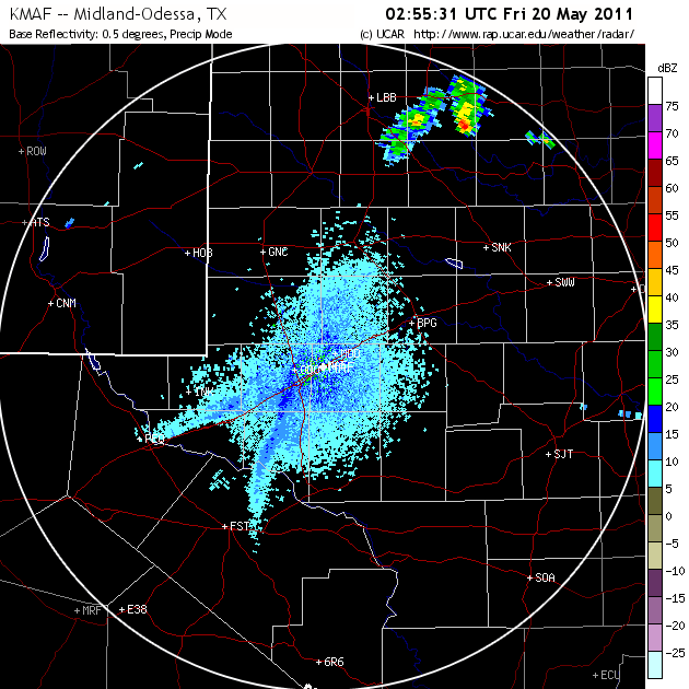
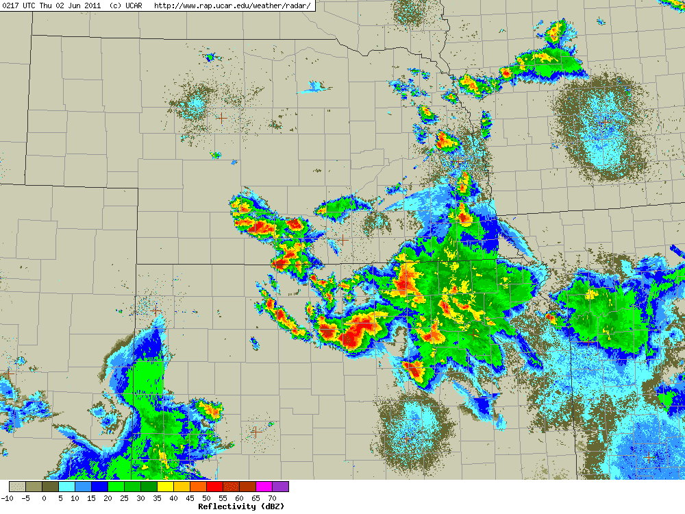
I will leave you with the current radar and ask quite simply: What will the radar look like in 3 hours?

displayN0R

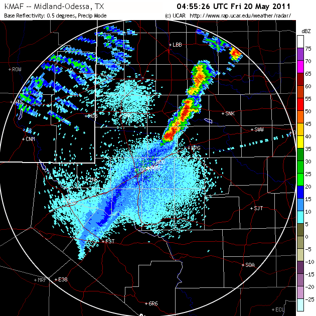
UPDATE: Here is what the radar looked like 3 hours later:

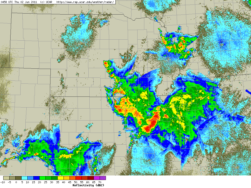
Nothing like our forecast for new storms. But that is the challenge when you are making forecasts like these.

Tags:

This week in CI

The week was another potpourri of convection initiation challenges ranging from evening convection in WY/SD/ND/NE to afternoon in PA/NY back over to OK/TX/KS for a few days. We encountered many similar events as we had the previous week struggling with timing of the onset of convection. But we consistently can place good categorical outlooks over the region, and have consistently anticipated the correct location of first storms. I think the current perception is that we identify the mechanisms and thus the episodes of convection, but timing the features remains a big challenge. The models tend to not be consistent (at least in the aggregate) for at least two reasons: There is no weather event that is identical to any other, and the process by which CI occurs can vary considerably.

The processes that can lead to CI were discussed on Friday and include:
1. a sufficient lifting mechanism (e.g. a boundary),
2. sufficient instability in the column (e.g. CAPE),
3. instability that can be quickly realized (e.g. low level CAPE or weak CIN or low LCL or small LFC relative to the LCL),
4. a deep moist layer (e.g. reduced dry air entrainment),
5. a weakening cap (e.g. cooling aloft).

That is quite a few ingredients to consider quickly. Any errors in the models then can be amplified to either promote or hinder CI. In the last 2 weeks, we had at least similar simulations along the dryline in OK/TX where the models produced storms where none were observed. Only a few storms were produced by the model that were longer lasting, but the model also produced what we have called CI failure: where storms initiate but do not last very long. Using this information we can quickly assess that it was difficult for the model to produce storms in the aggregate. How we use this information remains a challenge, because storms were produced. It is quite difficult to verify the processes we are seeing in the model and thus either develop confidence in them or determine that the model is just prolific in developing some of these features.

What is becoming quite clear, is that we need far more output fields to adequately scrutinize the models. However, given the self imposed time constraints, we need a data visualization system that can handle lots of variables, perform calculations on the fly, and deal with many ensemble members. We have been introduced to the ALPS system from GSD and it seems to be up to the challenge for the rapid visualization and the unique display capabilities for which it was designed (e.g. large ensembles).

We also saw more of what the DTC is offering in terms of traditional verification, object based verification, and neighborhood object based verification. There is just so much to look at it, that it is overwhelming day to day. I hope to look through this in the post experiment analysis in great detail. There is alot of information buried in that data that is very useful (e.g. day to day) and will be useful (e.g. aggregate statistics). This is truly a good component of the experiment, but there is much work to be done to make it immediately relevant to forecasting, even though the traditional impact is post experiment. Helping every component fill an immediate niche is always a challenge. And that is what experiments are for: identifying challenges and finding creative ways to help forecasting efforts.

Tornado Outbreak

I am posting late this week. It has been a wild ride in the HWT. The convection initiation desk has been active and Tuesday was no exception. The threat for a tornado outbreak was clear. The questions we faced for forecasting the initiation of storms were:
1. What time would the first storms form?
2. Where would they be?
3. How many episodes would there be?

This last question requires a little explanation. We always struggle with the criteria that denotes convection initiation. Likewise we struggle with how to define the multiple areas and multiple times at which deep moist convection initiates. This type of problem is “eliminated” when you issue a product for a long enough time period. Take the convective outlook for example. Since the risk is defined for the entire convective day you can account for the uncertainty in time by drawing a larger risk area and subsequently refining it. But as you narrow down your time window (from 1 day to 3 hours or even 1 hour) the problems can become significant.

In our case, the issue for the day was compounded because the dryline placement in the models was significantly east of the observed position by the time we started making our forecast. We attempted to account for this fact and as such had to adopt to a feature relative perspective of CI along the dryline. However, the mental picture you are assembling of the CI process (location, timing, number of episodes, number of storms) is tied not just to the boundaries you are considering, but the presumed environment in which they will form.

The feature relative environment then would necessarily be in error because we simply do not have enough observations to account for the model error. We did realize that shallow moisture, which was shown on morning soundings, was not going to be the environment in which our storms formed. Surface dew points were higher and staying near 68 in the warm sector. We later confirmed this with soundings at LMN which showed the moist layer increase in depth with time.

So we knew we had two areas of initial storm formation, one in the panhandle of OK and into KS along the cold front to the west and triple point to the east. The other area was along the dryline in OK and TX. We had to decide how far south storms would initiate. As we figuring all of this out, we had to look at the current satellite imagery since that was the only tool which was accounting for the correct dryline placement and estimate how far east it might travel, or mix out to in order to make the forecast.

Sure enough, the warm sector had multiple cloud streets ahead of the dryline. Our 4km model suite is not really capable of resolving cloud streets but we still needed to make our forecast roughly 1-2 hours before CI. So in a sense we were not making a forecast as much as we were making a longer more uncertain nowcast (probably not abnormal given the inherent unpredictability of warm season convection). Most people put the first storm in KS and would end up being quite accurate in placement. Some of us went ahead of the dryline in west central OK and were also correct.

There was one more episode in southern OK and then another in TX later on. This case will require some careful analysis to verify the forecast, other than subjective assessments. Today we got to see some of the potential objective methods via DTC, showing MODE plots of this case. The object identification of reflectivity via neighborhood and also merging and matching were quite interesting and should foster vigorous discussion.

Last but not least, the number of models we interrogated continued to increase, yet we were feeling confident in understanding this wide variety of models using all of the visualization tools including the more rapid web-based plots, and the use of the sub-hourly convectively active fields. We are getting quite good at distilling information from this very large dataset. There are so many opportunities for quantifying model skill that we will be busy for a long time.

It was interesting to be under the threat of tornadoes and to be in the forecast path of them. It was quite a day, especially since the remnant of the hook echo moved over Norman showering debris over the area picked up from the Goldsby Tornado. The NWC was roughly 3-5 miles away from the dissipation point of that Tornado.

Quick Post

I have blogged here about scales of CI but this weekend was a great example.
Saturday:

tlx

These storms formed in close proximity to the dryline where the southern most supercell went up pretty quickly and the other to the North and West went up much slower, remained small and then only the closest storm to the supercell formed into one. But the contrast is obvious. Even after breaking the cap, the storms remained small for an hour or so, and a few remained small for 2.

Today, we saw turkey towers along the dryline for quite a while (2 hours-ish) in OK and then everything went up. But it is interesting to see the different scales, even at the “cloud scale” where things tend be uneven and random, skinny and wide, slow and fast. It makes you wonder what the atmospheric structure is, especially when our tools tell us the atmosphere is uncapped, but the storms just don’t explode.

Looks like a pretty active southern Plains week is just beginning, as evidenced by the 43 tornado reports today and the 20 yesterday.

Tags:

Relative skill

During the Thursday CI forecast we decided to forecast for a late show down in western Texas where the models were indicating storms would develop. The models had a complex evolution of the dryline and moisture return from SW OK all the way down past Midland, TX. There was a dryline that would be slowly moving southeast and what we thought could be either a moisture return surge or bore of some kind moving northwest. CI was being indicated by most models with large spatial spread (from Childress down to Midland) and some timing spread (from 03 to 07 UTC) depending on the model. More on this later.

Mind you, none of these models had correctly predicted the evolution of convection earlier in the day along the TX panhandle-western OK border. In fact the dryline in the model was well into OK and snaked back southwest and remained there until after 23 UTC. The dryline actually made it to the border area, but then retreated after the storms formed southwest of SW OK in TX. This was probably because of the outflow from these storms propagating westward. This signal was not at all apparent in the models, maybe because of the dryline position. The storms that did form had some very distinct behavior with storms that formed to the north side of the 1st initiation episode moving North, not east like in the models. The southern storms were big HP supercells, slowly moving east northeast, and continually developing in SW OK and points further SW into TX (though only really the first few storms were big; the others were small in close proximity to the big storms – a scale enigma). We had highlighted the areas to the south in our morning forecast, along with an area in KS to the North but left a sight risk of CI in between. So while our distinct moderate risk areas would sort of verify in principle (being two counties further to the east than observed) we still did not have the overall scenario correct.

That scenario being, storms developing in our region and moving away, with the possibility for secondary development along the dryline a bit later. Furthermore we expected the storms to the north to develop in our moderate risk area and move east. When in fact the OK storms moved into our KS region just prior to our northern KS moderate area verifying well with an unanticipated arcing line of convection. This was a sequence of events that we simply could not have anticipated. We have discussed many times having the need to “draw what the radar will look like in 3 hours”. This was one of those days where we could not have had any skill whatsoever in accomplishing that task.

Drawing the radar in 1 or 2 or 3 hours is exactly what we have avoided doing given our 3 hour forecast product. We and the models, simply do not have that kind of skill at the scales where it will be required to have added value. This is not so much a model failure or even human failure. It is an operational reality that we simply don’t have enough time to efficiently and quickly mine the model data to extract enough information to make a forecast product. More on this later.

Back to the overnight convection. So once these SW OK supercells had been established we sought other model guidance, notably the HRRR from 16 or 17 UTC. By then it had picked upon the current signal and was showing a similar enough to observations evolution. This forecast would end up being the closest solution, but to be honest was still not that different way down in TX to the ensemble which was a 24-30 hour forecast. They all said the same thing: dryline boundary and moisture surge would collide, CI would ensue within 2 hours into a big line of convective storms that would last all night and make Fridays forecast very difficult.

Sure enough these boundary collisions did happen. From the surface stations point of view, winds in the dry air had been blowing SW all day with temps in the upper 80’s low 90s. After 02 UTC, the winds to the NW had backed and were now blowing W with some blowing W-NW. While at the dryline, winds were still SW but weakening. Ahead of the dryline, they were SE and weak. By 0400 UTC, the moisture surge intensified from weak SE winds to strong SE winds, with the dew point at CDS increasing from 34 to 63 in that hour. On radar the boundaries could be seen down in Midland, as very distinct with a clear separation:

maf

You can see CI already ongoing to the north where the boundaries have already collided and the zipper effect was in progress further southwest but it took nearly 2 more hours.

maf2

Also note the “gravity waves” that formed in the upper level frontal zone within a region of 100 knots of vertical shear back in NM. Quite a spectacular event. Let me also note that the 00 UTC ensemble and other models DID NOT pick up this event, until 3 hours later than shown by the last radar image. Spin up may have played a significant role in this part of the forecast. As you can see, the issues we face are impressive on a number of levels, spatial, and temporal scales. We verified our forecast of this event with the help of the ensemble and the HRRR and the NSSL WRF. To reiterate the point of the previous post: It is difficult to know when to trust the models. But in this case we put our faith in the models and it worked out, whereas in the previous forecast, we put our faith in the models and we had some relative skill, but not enough to add value.

Not so fast

What can I say. We verified our Tuesday forecasts and felt pretty good capturing the elevated convection over KS and OK at about the right time (1st lightning strike was 45 minutes before our period start time) for an elevated convection event and we rocked it out in CO during the day.

Which brings us to Wednesday. A slight risk in OK with a triple point from a warm front, stationary front and dryline in place. The dryline was forecast to be nice and strong, with horizontal convective rolls (HCRs) present on the north side interacting with the dryline circulation, and more HCRs in the dry air behind the dry line further south. The end result was a series of CI failures (indicated exclusively by accumulated precipitation) along the dryline, but eventually classic right moving supercells (1 or 2 dominant and long lived) were present in the ensemble. The HCRs were detected via some of the unique output variables we are experimenting with, particularly vertical velocity at 1.1 km AGL.

The complicating factor was that not all members had supercells, perhaps 1 in 3. We also had a situation where CI was very sensitive to the distribution of mixing ratio in the warm sector. It appeared we had two different behaviors along the dryline southward, but a definite moisture pool was dominant to the north. This pool was in the area where the dryline bent back westward and where the HCRs directly interacted with the dryline/warm front boundary. There was very little vertical velocity in the warm sector. Not sure why this was the case, assuming the PBL heights were not much lower than 1.1 km.

But lets be serious. There was not a whole lot of over-forecasting by the models. Storms did attempt to form. They just didn’t last very long or get very strong. Nor could we really call them storms (having met no single definition of CI other than some coherent weak reflectivity). In this case it appears the strongest forcing (the dryline and HCRs) was separated from where the realizable instability was present. We analyzed where, when, and how the instability could be realized (in great detail) in the model. We could not verify these models with observations because we don’t have very many sounding sites nor do we have frequent launches.  What we could not do is pinpoint where this forecast was going wrong.

The KOUN sounding is presented below:

OUN

Note that this sounding has nearly 3000 J/kg CAPE with 43 knot deep layer shear, and strong (31 knot) 0-1km shear. An ideal sounding for supercells, and possibly tornadoes. But Norman is well away from where the dryline was setup in western OK. There are no sounding sites in SW OK or NW OK. If we look at LMN which is north of OUN and happens to be north of the warm front:

lmn

We see very little instability because of cooler surface temperature and dew point and an elevated capped layer. Modifying this sounding for surface conditions at OUN would indicate strong instability and no cap using the virtual parcel. It is unlikely to be this easy as there is probably some mesoscale variability that has not been sampled in this area.

What is clear is that the forecasters were very much willing to buy into a reasonable solution. What we lacked was a solid reason to not believe the models. I am assuming we should first believe the models and that is perhaps not the best starting point. So lets reverse that thought: what reasons did we use to believe the models? I won’t speak for the group, but we should address this question when we review this event tomorrow.

Another point: Assume the model is not a poor representation of observations. What if it was very close? How could we recognize the potentially small errors which could lead to the development of storms or the lack there of? These are really fundamental questions that still need to be addressed.

On a day like today it would have been highly valuable to have soundings in key storm-scale locations near the dryline in the warm sector to the east, and to the immediate north between the dryline and warm front. At the very least we can ascertain if the model was depicting the stratification correctly and also the moisture content, instability and inhibition. It would have been great to have a fine scale radar to measure the winds around the dryline to look for HCRs.

Opportunities

Every Monday we get a new group of participants and this week we spent time discussing all the issues from their perspective. From an aviation, airport, and airplane perspective to towering cumulus from the mountains. We then discussed the forecast implications from verification, to model data mining, to practical use of forecast data and again learned the lesson that forecasters already know: you only have so much time before your forecast is due and it better contain the answer!

Our forecast has evolved into a 3 hour categorical product of convection initiation where we determine the domain and the time window. We then go a step further and forecast individually a location where we think the first storm will be in our domain during our time period. We then forecast the time we think it will occur and our uncertainty. Then we assign our confidence that CI will occur within 25 miles of our point. It might sound easy, but it takes some serious practice to spin up 10 people on observations, current and experimental guidance, AND lots of discussion about the scenario or scenarios at play. We have a pretty easy going group, but we do engage in negotiations about where to draw our consensus categorical risk and over what time period we are choosing. It is a great experience to hear everyone’s interpretation of the uncertainty on any number of factors at play.

Monday was a great practice day with a hurried morning forecast, and terrain induced CI forecast in the afternoon. Tuesday we were off to a good start with all products nominal, 10+ forecasters, and action back out on the Plains with plenty of uncertainty. The highlights from today included the introduction of ensemble soundings via the BUFKIT display (Thanks Patrick Marsh!). This garnered a lot of attention and will be yet another new, exciting, and valuable visualization tool. The aviation forecasters shared tremendous insights about their experiences and even showed a movie of what they face as airplane traffic gets shuffled around thunderstorms. It was a glimpse of exactly the sorts of problems we hope to address with these experimental models.

These problems are all associated with the CI problem, on every scale (cloud, storm, squall line scales). The movie highlighted the issue of where and when new convection would fill in the gaps, or simple occupy more available air space, or block and airport arrival, or when convection would begin to fizzle. Addressing these issues is part of the challenge and developing guidance relies almost exclusively on how we define convection initiation in the models and observations. We have some great guidance and it is clear that as we address more of the challenges of generic CI we will require even more guidance to account for the sheer number of possibilities of where (dx, dy and dz), when, how, and if CI occurs.

As an example, we issued our first night time elevated convection forecast. As it turns out, we could be verifying this by observing rain in OK tonight. Our experimental guidance was inadequate as we have very little data aloft except soundings from the fine resolution models. So we looked at more regular models while using what was available from the fine resolution models, like reflectivity and CI points. This highlights a unique operational challenge that we all face: Data overload and time intensive information extraction. The forecast verification for tonight should be quite revealing and should provide more insight than I am prepared to discuss this evening.

When seeing is believing

The HWT is examining some fairly sophisticated model simulations over a big domain. One question that frequently arises is: Can we trust the model over here if it is wrong over there?

What does “wrong” mean in these somewhat new models? Wrong in the sense that convection is absent or wrong in the sense that convection is too widespread? Perhaps, a particular feature is moving too slow or too fast. Can you really throw out the whole simulation if a part is “wrong”? Or do you just need time to figure out what is good/bad and extract what you can? Afterall the model is capable of detail that is not available anywhere else. That includes observations.

So Thursday and Friday we discussed how wrong the models have been. The features missed, the features misrepresented, the features absent. Yet each day we were able to extract important information. We were careful about what we should believe. On Friday, though, it was a different story. The NSSL WRF simulated satellite imagery was spot on. That is 14 hours into the simulation where the upper low, its attendant surface cold front were almost identical.

Our domain was northern AR, southern MO, western TN and MS. The models were not in agreement mind you. The different boundary layer schemes clustered into two groups: all the schemes were going for the northern AR initiation, and a second group, the TKE based schemes were also going for the southern part of the cold front. Another signal I was paying attention was post-frontal convergence that was showing up. I made note of it but I never went back to check all the simulations but I wanted to keep that threat in the forecast. Turns out, the TKE schemes hit on all of these features. The northern storms initiated similar to model consensus, the southern storms initiated as well, and so did the secondary episode behind the front (at least from the radar perspective). 

The second domain of the day was Savannah GA, in the afternoon. This was an event involving convection possibly moving in from the west, the sea breeze front penetrating far inland along the east, a sea breeze fron the west FL and gulf coast sea breeze penetrating even farther inland, and a highly organized boundary layer sandwiched in between. The models had little in the way of 30 dBz 1km reflectivity at hourly intervals. The new CI algorithms showed that CI was occurring along all of the aforementioned features:
1. Along the sea breezes,
2. in the boundary layer along horizontal convective rolls,
3. along the intersections of 1 and 2,
4. and finally along the outflow entering into our domain.

We went for it and there was much rejoicing. We watched all afternoon as those storms developed along radar fine lines, and along the sea breeze. This was a victory for the models. These storms ended up reaching severe levels as a few reports came in.

As far as adding value on days like this, I am less certain. Our value was in extracting information. There is much to add value to. At this stage, we are still learning. It is impossible to draw what the radar will look like in 3 hours (unless there is nothing there). But I think as we assemble the capabilities of these models, we will be able to visualize what the radar might look like. As our group discussed, convection in the atmosphere appears random. But only because we have never seen the underlying organization.

It is elusive because our observing systems do not see uniformly. We see vertical profiles, time series at a location, and snap shots of clouds. We see wind velocity coming towards or away from radars. We see bugs caught in convergence lines (radar fine lines). So these models provide a new means to see. Maybe we see things we know are there. Maybe we are seeing new things that we don’t even know to look for. Since we can not explain them we are not looking for them. We expect to see more cool stuff this week.

Thanks to all the forecasters this week who both endured us trying to figure out our practical, time limited forecast product, and who taught us how to interrogate their unique tools and visualizations. We begin anew tomorrow with a whole new crop of people, a little better organized, with more new stuff on display, and more complex forecasts to issue.