Well today the severe weather forecast area was from eastern CO and western KS. Although the hi-res models were producing some intense precipitation cores it was highly unlikely the atmosphere would follow suit. The deep dry boundary layer would be capable of supporting some serious downdrafts but without a lot of moisture, wet downbursts were unlikely. However, dry thunderstorms were the possible convective mode and all available evidence hinted at a line that would fizzle later in the evening.

Severe reports from KS showed up just prior to 0000 UTC right along with an OK mesonet wind gust to 58 mph. Now normally when you get a downdraft, it brings cooler air to the surface. In the case of a deep and dry boundary layer, there can be little in the way of temperature changes. This is exactly what occurred with the temperature going slightly up 4F during the big wind gust!

I went out on a limb and also proceded to forecast a 20 percent chance of heatbursts. A few models hinted at that possibility tonight (in the next few hours anyway). Verification in the morning!

So after much discussion today about moisture there is accumulating evidence. Here is a comparison between the MWR on the roof (1.6cm at 00 UTC 5/17 and 2cm at 00 UTC 5/18) , the IPW from the GPS system (gpsmet.noaa.gov), and the radiosonde launch from Norman.
GPS:

Here is the sounding:

Note the PW is 0.5″ with a characteristic decrease immediately off the surface. Just after this time the dew point at the NWC increased from 53 to 55 in the hour after release.

Below is the MWR PW time series with the last vertical dotted line at the right being 0000 UTC on 5/18 (the beginning of the chart is 5/17 at 00 UTC):

The MWR agrees well with the GPS system and the MWR is fresh off a calibration. I have no idea what would cause this discrepancy with the radiosonde data but clearly something is amiss.

Let me back up to DVN on the 16th at 0000 UTC for a counter example:

And now the corresponding GPS data from Rock Island:

Note the close correspondence for a few balloon launches; specifically at 5/16 00 UTC! Yet that decrease above the surface looks suspect. It is possible the cloud layer above 700 mb is laying a role but what I don’t think we can diagnose.

The models stole it all!

One of the additions this year is an observational program (brought to you by NSSL) where we have an Microwave Radiometer (MWR) offering vertical profiles of moisture and temperature over the lowest 4km AND a new radiosonde intercomparison to go along with it (a Vasaila RS92 sonde and a new IMET sonde). The goal is to use the soundings to compare the MWR and thus offer a calibration data set, but also to see how well the moisture retrievals compare to actual, in clear-sky conditions.

Since we have had two sonde launches this week so far we can see how well the IMET and Vasiala measurements compare and also how the MWR compares to both of them. So far the results are that the two sondes are very close. The comparison with the MWR was at first horrible, until the MWR was re-calibrated. Sensor drift from one of the eight channels was to blame at least for the low level structure of the moisture (most noticeable in the RH field). for the next point we have to understand that the majority of the information content in the moisture channels is contained below 4km and only amounts to about (on average) 1.6 pieces of information. This means within the lowest 4 km we have at most 2 effective measurement points for moisture. So the vertical profiles tend to be smooth and more like an average which is why agreement aloft between moist layers and the MWR is essentially low.

OK has been pretty low on moisture the last couple weeks. We spent some time forecasting in the Iowa area the other day where model precipitable water was in excess of 1″, but in reality was only around 0.5″. This posed no problems for the models to generate storms along a cold front associated with an upper low. Some warnings resulted from MI arcing through IA that evening with a few wind and hail reports, but generally good CI and SVR forecasts.

At issue was this anomalous model moisture and if/how it would play a role in the forecast. So many models had storms though that it was hard to discount storms even in this lower moisture environment. Even looking back at the verifying soundings from DVN, ILX, DTX it was evident that the CAPS ensemble control member was 2-3 g/kg too moist through the depth of the boundary layer. How can we have errors that large and yet have some skill in the convective forecasts? The models simulated storms were a bit on the high side in terms of reflectivity, lasted a bit longer, were a bit larger, but still had similar enough evolution. I guess you could consider this a good thing, but this should really drive home the point that better, more dense moisture observations are needed.

We really need to see WHY these errors occur and diagnose what is contributing to them. In this case, the control member was an outlier in terms of the overall ensemble. Why? Was it the initial conditions, lateral boundary conditions, the perturbations applied to the ensemble members, or some combination thereof that set the stage for these differences in convection? Or was it the interplay between the various model physics and all previous factors? We will need to dig deep on this case to get any kind of reasonable, well constrained answer.

In order to address, at least partially, these issues we need observations of moisture within the PBL. In fact we could even benefit from knowing the boundary layer. It is at least plausible to retrieve that field and then derive the PBL moisture. Such is the goal of the MWR type of profiler: to derive the lowest layer moisture structure, addressing at least some of our issues. Regardless, these high resolution models REQUIRE observations to verify both the processes and statistics of these models in order to make improvements.

I am really behind on the blog posts. Last week had some challenges especially for severe storms down in south Texas. We have had a few days where the cutoff lows have been approaching south Texas providing sufficient vertical shear and ample moisture and instability. The setup was favorable but our non-met limitation was the border with Mexico. We don’t have severe storm reports in Mexico nor do we have radar coverage. Forecasting near  a border like this also  imposes a spatial specificity problem. In most cases there is room for error, room for uncertainty especially with making longer (16 hr) spatial forecasts of severe weather. On one particular day the ensemble probabilities were split: 1 ensemble in the US with extension into Mexico, 1 ensemble in Mexico with extension into the US, and another further northwest split across the two unevenly into the US. 

So the challenge quickly becomes all about specificity … where do you put the highest probabilities and where are the uncertainties large (i.e. which side of the border).  The evolution of convection quickly comes into question also since as you anticipate where the most reports might be (where will storms be when they are in the most favorable environment), you have to also account for if/when storms will grow upscale, how fast that system will move and if it will also be favorable to generate severe weather.

We have discussed this in previous experiments as such: “Can we reliably and accurately draw what the radar will look like in 1, 3, 6, 12, etc hours?”. This aspect in particular is what makes high-resolution guidance valuable. It is precisely a tool that offers what the radar will look like. Furthermore, an ensemble of such guidance offers a whole set of “what if” scenarios. The idea is to cover the phase space so that the ensemble has a higher chance of depicting observations. This is why taking the ensemble mean tends to be better (for some variables) than any individual member of an ensemble.

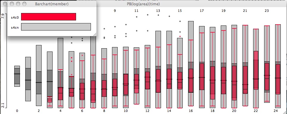
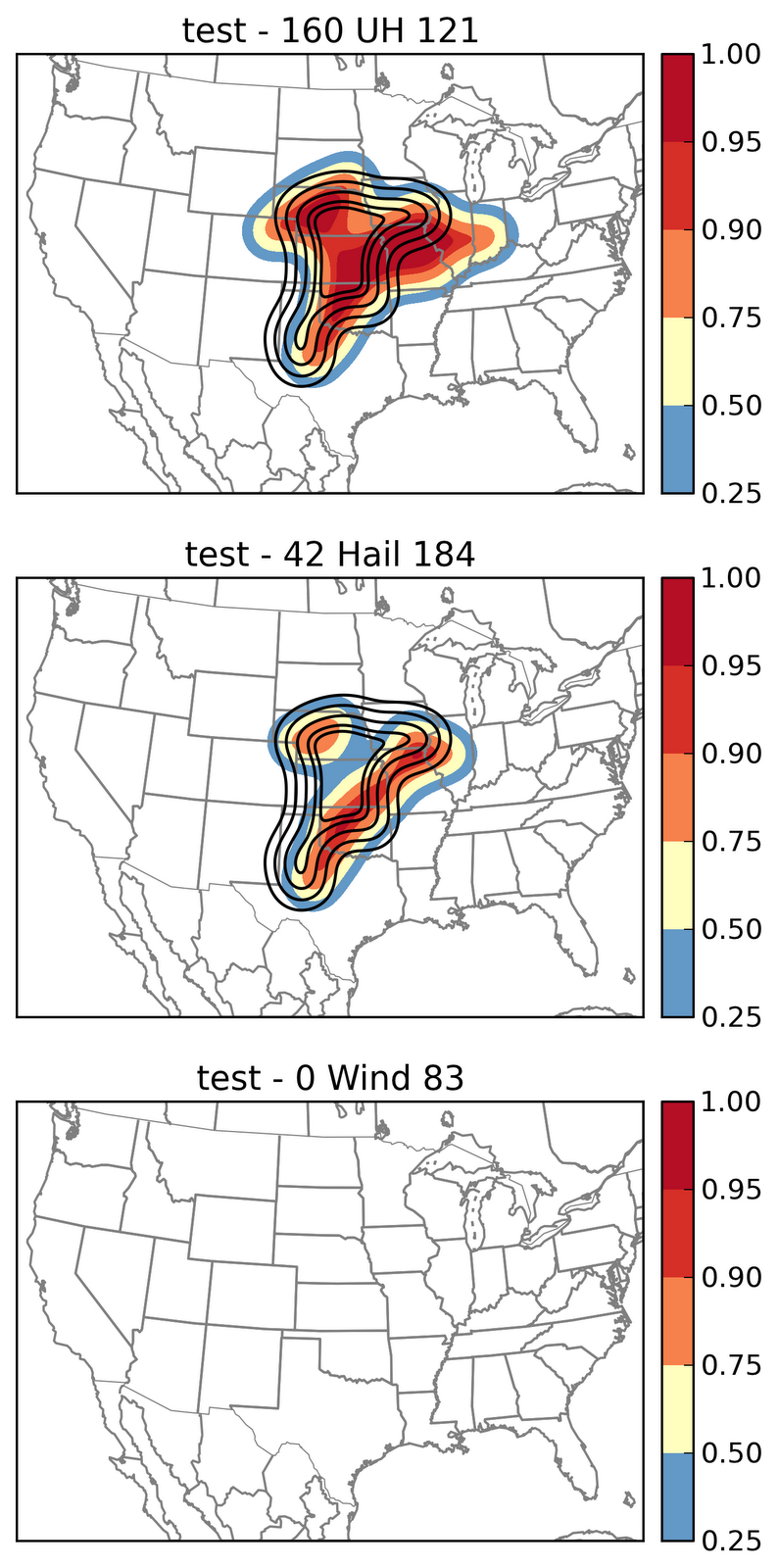
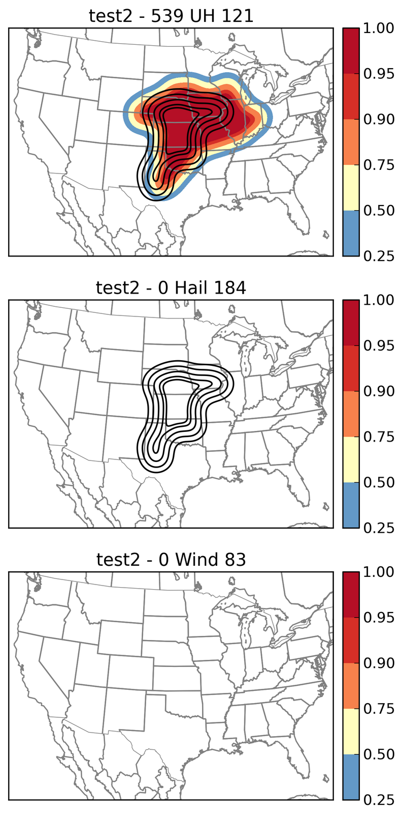
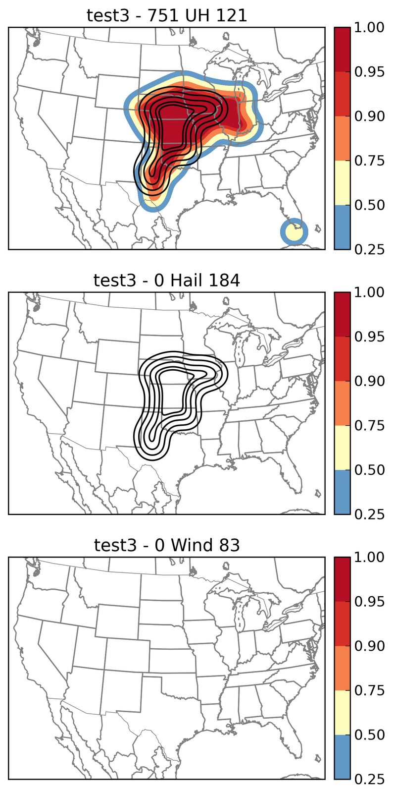
 Utilizing all these members of an ensemble can become overwhelming. In order to cope with this onslaught (especially when you 3 ensembles with 27 total members), we create so-called spaghetti diagrams. These typically involve proxy variables for severe storms. By proxy variables I mean model output that can be correlated with the severe phenomenon we are forecasting for. This year we have been looking at simulated Reflectivity, Hourly maximum (HM) storm updrafts, HM updraft helicity, and HM wind speed. Further, given the number of ensembles, we have so-called “buffet diagrams” where each ensemble is color coded but now depicts each and every member. We have also focused heavily on probabilities for each of the periods we have been forecasting for.

In this case all the probabilities are somewhat uncalibrated. Put another way the exact value of the probabilities do not corresponding directly to what we are forecasting for nor have we incorporated how to map them from model world to the real world. In one instance we do have calibrated ensemble guidance but not for the 2 other ensembles. It turns out you need a long data set to perform calibration for rare event forecasting like severe weather.

Lets come back to the forecasts. Given that each ensemble had a different solution it was time to examine if we could discount any of them given what we thought was a likely scenario. We decided to remove one of the ensembles from consideration. The factors that led to this decision were a somewhat displaced area of convection that did not match observations prior to forecast time, and a similar enough evolution of convection. It was decided to put some probabilities in the big bend area of Texas to account for early and ongoing convection. This was a relatively decent decision as it turned out.

This process took about 2 hours and we didn’t really dig into the details of any individual model with complete understanding. Such are the operational time constraints. there was much discussion on this day about evolution. Part of the evolution was the upscale growth (which occurred) but also whether that convection produced any severe reports. Since the MCS that formed was almost entirely in Mexico, we won’t know whether severe weather was produced. Just another day in the HWT.

Today was an interesting day as we had a joint decision to pick our domain of where we would collectively issue our forecasts. It was decided the clean slate CI and severe domain would be in south Texas. According to the models this area would potentially result in multiple types of potential severe weather (outside the stronger flow pulse severe was possible and further north in the frontal zone area, possible behind, where the flow and shear were stronger, more organized threat) as well as multiple triggers for CI (along the cold front moving south, the higher terrain in Mexico into NM, as well as potential along the sea breeze near Houston).

It was increasingly clear that adding value, by moving from course to high temporal resolution, is difficult because of how accurate we are requiring the models to be. The model capability may be good by simulating the correct convective mode and evolution, but getting that result at the right time and in the right place, will still determine the goodness of the forecast. So no matter the kind of spatial or temporal smoothing we apply to derive probabilities we are still at the mercy of the processes in the model that can be early or late and thus displaced, or displaced and increasingly incorrect in timing. This is not new mind you, but it underscores the difference between capability and skill.

In the forecast setting, with operational timeliness requirements, there is little room for only capability. This is not to say that such models don’t get used, it just means that they have little utility. The operational forecasters are skilled with available guidance so you can’t just put models with unknown skill in their laps and expect it to have immediate high impact (value). The strengths and weaknesses need to be evaluated. We do this in the experiment by relating the subjective impressions of participants to objective skill score measures.

And we do critically evaluate them. But let me be clear. Probabilities never tell the whole story. The model processes can be as important to generating forecaster confidence in model solutions. This is because the details can be used as evidence to support or refute processes that can be observed. Finding clues for CI is rather difficult because the boundary layer is the least well observed. We have surface observations which can be a proxy for boundary layer processes, but not everything that happens in the boundary layer happens at the surface.

A similar situation happens for the severe weather component. We can see storms by interrogating model reflectivity but large reflectivity values are not highly correlated with severe weather. We don’t necessarily even know if the rotating storms in the model are surface based which would yield a higher threat than say elevated strong storms. Efforts to use additional fields as conditional proxies with the severe variables are underway. These take time to evaluate and refine before we can incorporate them into probability fields. Again these methods can be used to derive evidence that a particular region is favored or not for severe weather.

Coming back to our forecast for today there was evidence for both elevated storms and surface based organized storms, and evidence to suggest that the cold front may not be the initiator of storms even though it was in close proximity. We will verify our forecasts in the morning and see if we can make some sense out of all the data, in the hopes of finding some semblance of signal that stands out above the noise.

Today is the first official day of the Hazardous Weather Testbed Experimental Forecast Programs’ Spring Experiment. We will have two official desks this year: Severe and Convection Initiation. Both desks will be exploring the use of high-resolution convection-permitting models in making forecasts which include on the severe side, the total severe storms probabilities of the Day 1 1630 convective outlook and then 3 forecast periods similar to the enhanced thunder (20-00, 00-04, and 04-12 UTC), while on the CI side they will make forecasts of CI and convection coverage for 3 four periods (16-20,20-00, 00-04 UTC).

We have 3 ensembles that will be used heavily: the so-called Storm Scale ensemble of opportunity (SSEO; 7 member including the NSSL-WRF, NMM-B Nest, and the hi-res window runs including 2 time lagged members), AFWA (Air Force 10 member), and SSEF (CAPS 12 member).

We will be updating throughout the week as events unfold (not necessarily in real time) and will try to put together a week in review. Let the forecasting begin.

I am debugging and modifying code to complement some of our data assimilation (DA) evaluations. In recent years efforts have been made to provide higher temporal resolution of composite reflectivity. I wanted to take a more statistical visualization approach to these evaluations. One way to do that is to data mine using object based methods, in this case storm objects. I developed an algorithm to identify storms using composite reflectivity using a double area double threshold method using the typical spread-growth approach. The higher temporal resolution of 15 minutes is good enough to identify what is going on in the beginning of the simulations when one model has DA and the other does not; everything else is held constant.

Among the variables extracted are maximum composite reflectivity, maximum 1km reflectivity, and pixel count for each object at every 15 minute output time. In order to make the upcoming plot more readable I have taken the natural log of the pixel count (so a value around 4 equates to 54 pixels, roughly speaking). The plot is a conditional box plot of ln(pixel count) by model time step with 0 being 0000 UTC and 24 being 0600 UTC. I have used a technique called linked highlighting to show the model run using data assimilation in an overlay (top). Note that the model without DA does not initiate storms until 45 minutes into the simulation (bottom). The take away point here being the scale at which storms are assimilated for this one case (over much of the model domain) at the start time is a median of 4.2 (or roughly > 54 pixels) while when the run without DA initiate storms they are on the low end with a median of 2.6 (13 pixels).

This is one aspect we will be able to explore next week. Once things are working well, we can analyze the skill scores from this object based approach.

Here are the NSSL(top), SSEO_0000 (middle), and SSEO_1200 (bottom) plots showing the model reports overlaid with the observed reports so far. The SSEO lacks hail and wind. Red dots indicate current observed storm reports. Black contours can be compared directly to he shaded model fields. The ensemble plots have 7 and 4 members, respectively. All go through 1200 UTC tomorrow morning.

UPDATE 1: I have rerun the graphics and they are displayed below.
NSSL-WRF (only looking at the top panel of “test”) compares favorably to the observations, at least in this smoothed representation. It does appear to be shifted too far east and south (the slight offset in the outer contours relative to the shading). But it did not capture the concentrated area of tornadoes in central KS. Despite “looking good” I think the skill scores would be somewhat low. I will try to run the numbers this week for all the models displayed so that each individual model can be compared and we can see which one, if any, stood out from the pack.

The SSEO ensembles are below: