
The capping tilt is determined by reading in subsequent tilts of the radar until a tilt is found in which none of the pixels have a reflectivity greater than a user-defined threshold, set with the -m flag. The algorithm then considers this tilt the cap, and does not read any tilts above this cap. The algorithm then runs, reading in all tilts below and including the capping tilt. This continues until either a) another capping tilt is found below the current capping tilt, or b) a pixel is found in the current capping tilt with a reflectivity greater than the threshold specified by the -m flag.
If a new capping tilt is found below the current capping tilt, the algorithm will then reads only the tilts below the new capping tilt. If a pixel is found to exceed the reflectivity threshold in the current capping tilt, the algorithm resumes reading all tilts until it finds another tilt with in which the reflectivity does not exceed the threshold in any pixel, and a new capping tilt is declared.
By specifying a threshold with the -m flag, you are basically telling the algorithm that you are not interested in any echoes below this threshold. You are also assuming that if there are no pixels in which the reflectivity exceeds the threshold in a particular tilt, there are also no pixels in which the reflectivity exceeds the threshold in the tilts above.
Finally, if you are interested in only rain rates, you can set the -E flag to further reduce the time it takes this algorithm to run. Rain rates are determined by examining the pixels nearest to the ground. In a perfectly flat world, we could read in and process only the lowest tilt from the radar and greatly reduce the processing time. However, we know that our world is not perfectly flat, and that many radars have terrain blocking some of the radials at the lower tilts. For these radials blocked by terrain, we need to find the next lowest unblocked radial. Therefore, we have devised a method in which we can determine the lowest tilt unblocked by terrain for each radar. Once this tilt is determined, only data below and including that tilt needs to be processed.
You can specify that you would like to process only up to the lowest unblocked tilt by setting the -E flag to the lowest elevation angle scanned by your radar (0.5 in the case of the WSR-88D network). This needs to be specified so the algorithm knows at which elevation to start looking for the lowest unblocked tilt.
So, if you are interested in only rain rates from a radar in the WSR-88D network, your command would look like:
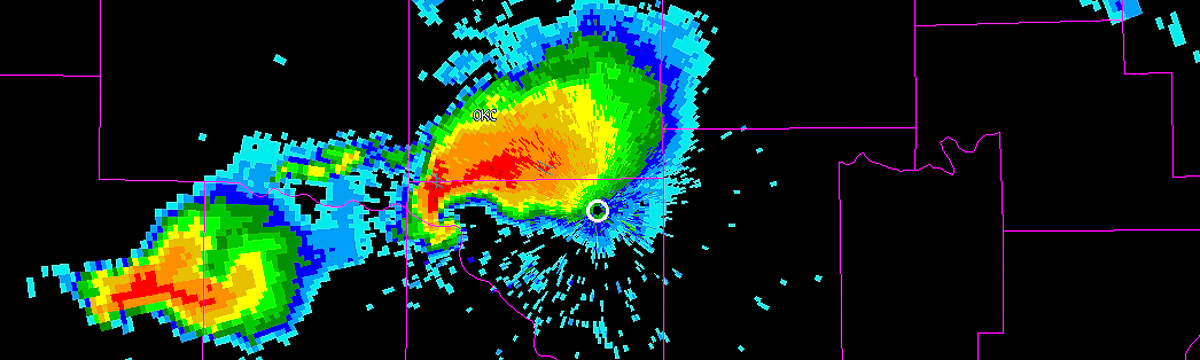
w2dualpol -i /data/KTLX/code_index.fam -o /data/KTLX -s KTLX -m 10 -E 0.5 -T /data/terrain/KTLX.nc --outputProducts=RREC
Notice that along with the -E flag, the -T flag is also set, specifying the terrain file for your radar. Additionally, the -m flag is set to 10, specifying that the capping elevation be set as the lowest elevation in which no pixels exceed 10 dBZ.
It should be noted that if you’re interested in processing some products at all elevations (say, HCA and MSIG), but the rain rates at only the lowest unblocked elevation, you will want to run two iterations of w2dualpol in order to process the data in the least amount of time.
First:
w2dualpol -i /data/KTLX/code_index.fam -o /data/KTLX -s KTLX -0 1 -m 10 -T /data/terrain/KTLX.nc --outputProducts=DHCA,MSIG
and then:
w2dualpol -i /data/KTLX/code_index.fam -o /data/KTLX -s KTLX -m 10 -E 0.5 -T /data/terrain/KTLX.nc --outputProducts=RREC
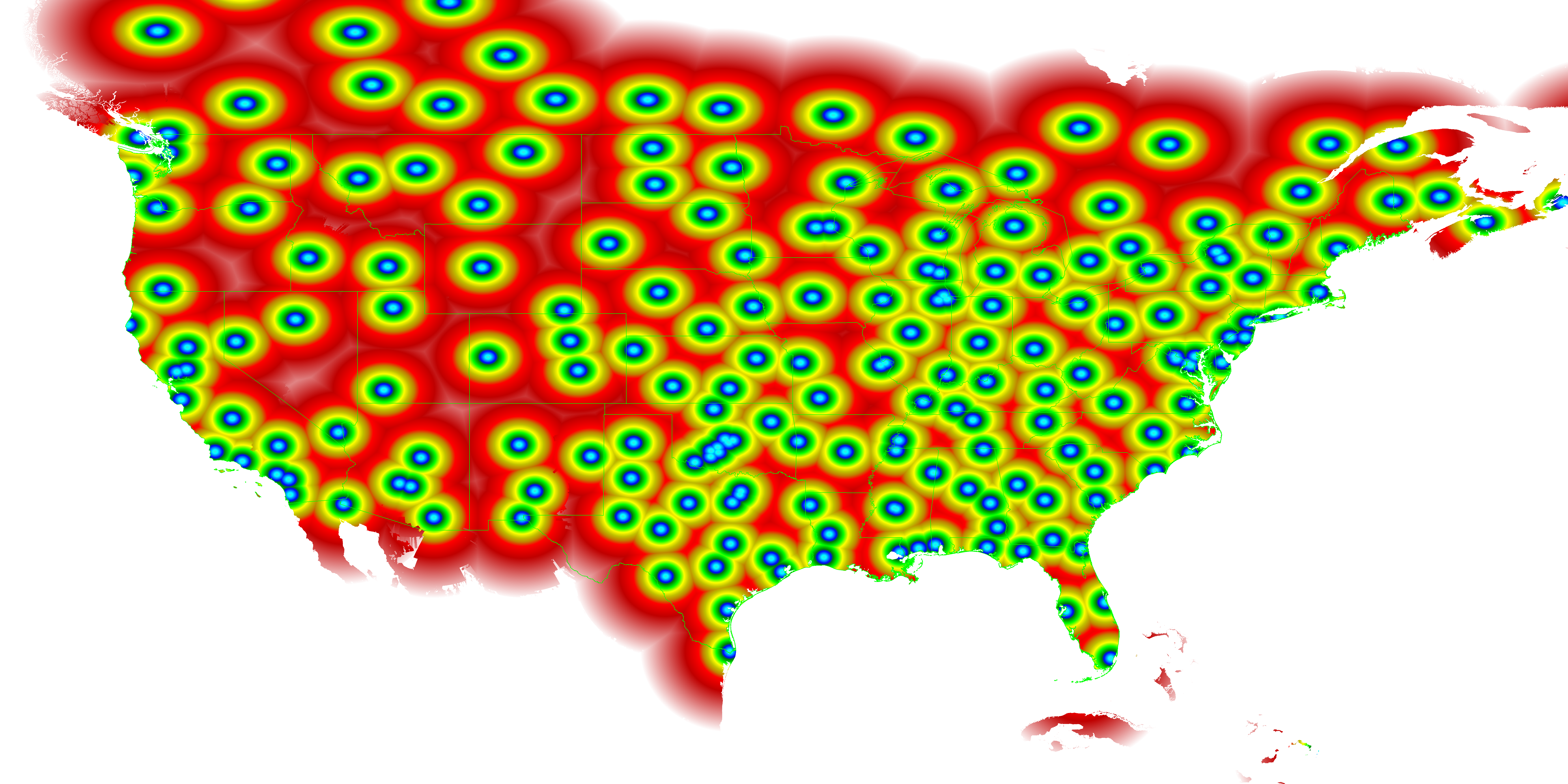
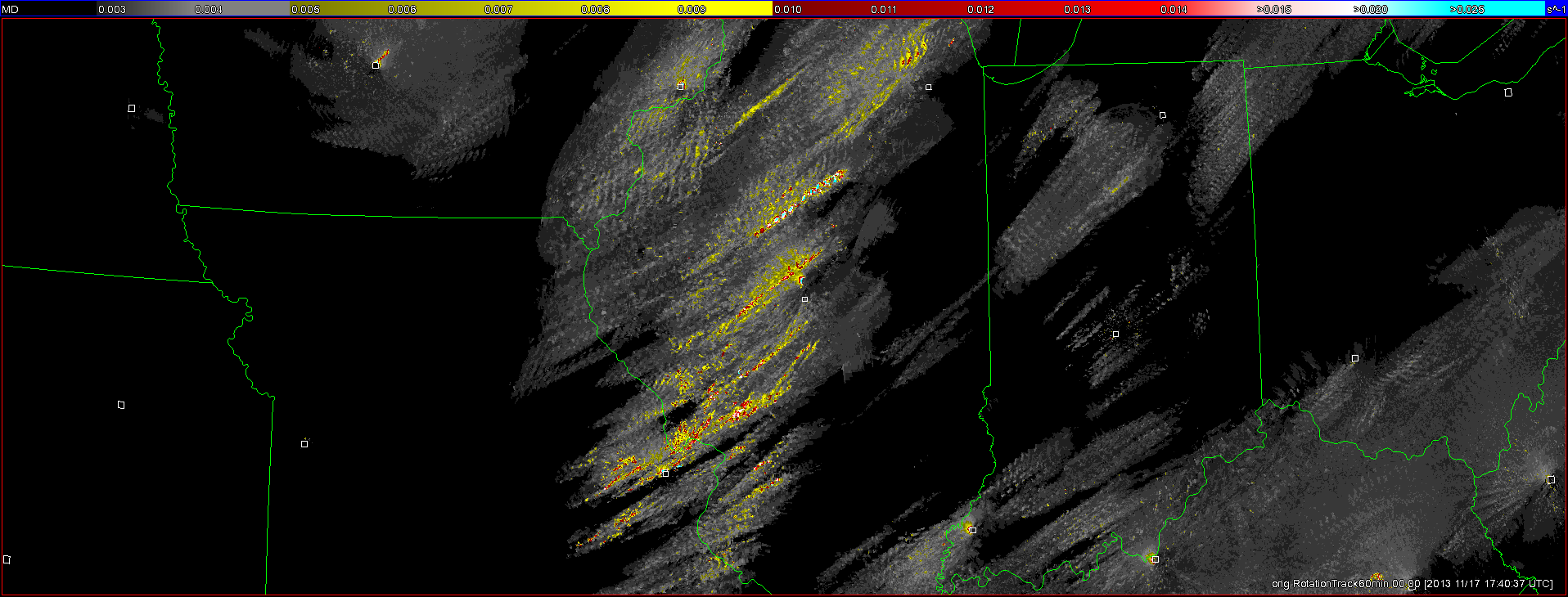
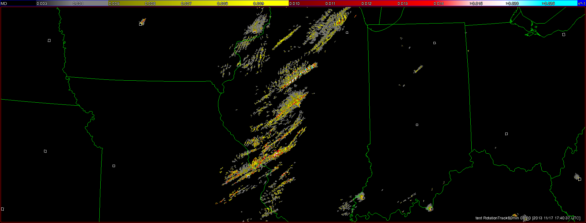
Through the implementation of the capping elevation and the lowest unblocked elevation, we are able to halve the processing time of w2dualpol. This means that the processing time is about 1/4 of that of the original ports of the ORPG algorithms, discussed in the previous post.

