Determining how closely a forecast matches what happens in reality is a crucial step in the evaluation of any type of forecast. Gridded forecasts, which are of particular interest to WDSS-II users, are no different. With this in mind, we will cover a method in WDSS-II to compare gridded forecasts to gridded observations. To make this comparison, we will make use of the algorithm w2scoreforecastll, which creates scores for the gridded forecasts based on how well they match observations.
More generally, w2scoreforecastll is used to compare two supposedly equivalent 2D fields (e.g., a forecast field and an observation field). The algorithm quantifies just how different the two fields are through an error score. When the error score is low, the two grids match well, meaning that the forecast did a good job of approximating reality.
In w2scoreforecastll, there are 4 different methods by which you can generate scores for your forecasts:
- Pixel By Pixel: Just comparing the values in corresponding pixels in each grid
- Object By Object: Used to score forecasted objects (e.g., storms)
- Gaussian Mixture Models: Described below
- Probabilistic: Used to score probabilistic forecasts
In many instances, the best option for scoring gridded forecasts is option number 3, Gaussian Mixture Models. This method is outlined in great detail in V. Lakshmanan and J. Kain, A Gaussian mixture model approach to forecast verification, Wea. Forecasting, vol. 25, no. 3, pp. 908-920, 2010.
In a nutshell, this algorithm approximates both the forecasted and observed grids with a mixture of Gaussians. Based on the parameters of these Gaussians, the algorithm computes 3 different measures of error: 1) translation error, 2) rotation error, and 3) scaling error. These errors are then all incorporated into one measure of error for the forecast, the combined error.
These error scores are computed at 8 different spatial scales. At the coarsest scale, the grids are approximated by just 1 Gaussian. Then, at subsequently finer scales, the number of Gaussians used to approximate the grids increases roughly exponentially to about 128 Gaussians at the finest scale.
As an example, lets say we are interested in seeing how close the 180 minute composite reflectivity from the High Resolution Rapid Refresh (HRRR) numerical forecast model gets to reality (here, we will say that the merged composite reflectivity from the WSR-88D network is reality). To do this, just use the command:
w2scoreforecastll -i /localdata/20130613/score_index.xml -o /localdata/20130613/HRRR/180minute/score.out -T "MergedReflectivityQCComposite:00.00 -F MaximumComposite_radar_reflectivity:180Minute -t 180 -m 3 -R Tracked
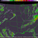
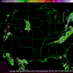
Be sure that your input index is pointing to both the forecast (HRRR) and observed (radar) fields. The algorithm will then take all 180 min HRRR forecasts, as well as all of the radar observations, and approximate those images with Gaussians, as shown in the figures below. The algorithm will then generate error scores for corresponding HRRR and radar grids and output the scores to the file specified in the -o option of the command line.
*Note: It is important to be sure that the domains of your two grids match. This can be easily done with w2socreforecastll. Simply specify which grid you would like the other to be remapped to with the -R flag in the command line. In the images above, the HRRR field was remapped to match the domain of the radar field, and then the Gaussians were created.
An excerpt of the output file form w2scoreforecastll is below:
<iteration number="17" forecast_time="20130613-170000" target_time="20130613-200000" timedifference="180">
 <gmmComparisionScore translation_error="0.145385" rotation_error="0.00267211" scaling_error="0.51418" combined_error="0.30124" num_gmm="1"/>
 <gmmComparisionScore translation_error="0.420869" rotation_error="0.00603904" scaling_error="0.140152" combined_error="0.197544" num_gmm="2"/>
 <gmmComparisionScore translation_error="0.294767" rotation_error="0.364796" scaling_error="0.337474" combined_error="0.330126" num_gmm="6"/>
 <gmmComparisionScore translation_error="0.375277" rotation_error="0.0519002" scaling_error="0.159446" combined_error="0.202686" num_gmm="8"/>
 <gmmComparisionScore translation_error="0.173481" rotation_error="0.0684976" scaling_error="0.226473" combined_error="0.17898" num_gmm="18"/>
 <gmmComparisionScore translation_error="0.251112" rotation_error="0.394195" scaling_error="0.0955482" combined_error="0.201947" num_gmm="35"/>
 <gmmComparisionScore translation_error="0.231869" rotation_error="0.3287" scaling_error="0.072619" combined_error="0.17161" num_gmm="69"/>
 <gmmComparisionScore translation_error="0.14816" rotation_error="0.18702" scaling_error="0.0419667" combined_error="0.102835" num_gmm="137"/>
</iteration>
Going through this output, we first see that we are on iteration number 17, where each iteration is associated with a new timestep. Next we see that we are comparing the 180 minute HRRR created at 20130613-170000 and the radar composite reflectivity at 20130613-200000. Finally we have the error scores for each scale. There is a section of the output file like the one above for each timestep. At the end of the file, all of the error score are aggregated (not shown).
This type of information is particularly valuable in situations where you want to compare different forecasts. Perhaps you want to know if at a particular forecast hour, you get a better forecast from advecting radar data forward in time or from the HRRR. With w2scoreforecastll, you can score both forecasts to determine which one is better.


