w2clustertable: a way to track storm properties over time

w2segmotionll provides a way to identify storm cells and track their properties over time so as to data mine storm attributes.  But w2segmotionll is not the best place for that functionality because:

  1. w2segmotion is also used to estimate motion from clusters, so as to create image nowcasts (using w2advector).  Adding storm attribute generation makes w2segmotion a performance hog in real-time applications.
  2. Storm tracking should not be limited to w2segmotion’s way of identifying clusters. Any object-identification method (not just the enhanced watershed approach we use) should be supported.

Following the WDSS-II philosophy, therefore, the cluster-table functionality of w2segmotion has been split off into a new program called w2clustertable.  Instead of providing the -X option to w2segmotion, pass the XML file into the -X option of w2clustertable.

w2clustertable also takes, as input, a label grid (the “KMeans” output of w2segmotion) and motion estimates (the Motion_East and Motion_South) outputs of w2segmotion.  But you could also use w2imgmotion to obtain cross-correlation-based motion estimates. And you can use any scheme to create a labeled set of storms (1,2,3…) to get their properties. It is not necessary for storm#4 in one frame to be storm#4 in the next frame (i.e., w2clustertable will associate storms using centroid-match or overlap or one of several built-in association methods).

If you use w2clustertable, please continue to cite our 2009 J. Tech paper:  V. Lakshmanan and T. Smith, “Data mining storm attributes from spatial grids,” J. Ocea. and Atmos. Tech., vol. 26, no. 11, pp. 2353-2365, 2009


With this change, here are some related programs in the storm identification and tracking realm:

  1. w2segmotionll uses K-Means clustering and Enhanced Watershed to identify storm cells at multiple scales.
    (see: V. Lakshmanan, K. Hondl, and R. Rabin, “An efficient, general-purpose technique for identifying storm cells in geospatial images,” J. Atmos. Oceanic Technol., vol. 26, no. 3, pp. 523-37, 2009)
  2. w2segmotionll uses these storms to compute motion estimates  (see: V. Lakshmanan, R. Rabin, and V. DeBrunner, “Multiscale storm identification and forecast,” J. Atm. Res., vol. 67, pp. 367-380, July 2003.)
  3. w2segmotionll and w2clustertable can both be used to track storm cells over time (see: V. Lakshmanan and T. Smith, “An objective method of evaluating and devising storm tracking algorithms,” Wea. Forecasting, vol. 25, no. 2, pp. 721-729, 2010.), but w2clustertable is now preferred.
  4. w2segmotionll and w2clustertable can both be used to compute storm attributes but w2clustertable is now preferred. (see: V. Lakshmanan and T. Smith, “Data mining storm attributes from spatial grids,” J. Ocea. and Atmos. Tech., vol. 26, no. 11, pp. 2353-2365, 2009)
  5. w2segmotionll and w2advectorll can both be used to create nowcasts of other fields from motion estimates obtained by tracking storms on one field but w2advectorll is the preferred way to do that. (see: V. Lakshmanan, R. Rabin, and V. DeBrunner, “Multiscale storm identification and forecast,” J. Atm. Res., vol. 67, pp. 367-380, July 2003.)
  6. w2flatten will take the multiscale cluster table output by either w2segmotionll or w2clustertable and “flatten” it into a single table, to make multi-scale data mining possible (forthcoming paper by Humphrey, Lakshmanan, Smith, Smith and Thompson).


Tags: None

Using GMMs to score gridded forecasts with w2scoreforecastll

Determining how closely a forecast matches what happens in reality is a crucial step in the evaluation of any type of forecast. Gridded forecasts, which are of particular interest to WDSS-II users, are no different. With this in mind, we will cover a method in WDSS-II to compare gridded forecasts to gridded observations. To make this comparison, we will make use of the algorithm w2scoreforecastll, which creates scores for the gridded forecasts based on how well they match observations.

More generally, w2scoreforecastll is used to compare two supposedly equivalent 2D fields (e.g., a forecast field and an observation field). The algorithm quantifies just how different the two fields are through an error score. When the error score is low, the two grids match well, meaning that the forecast did a good job of approximating reality.

In w2scoreforecastll, there are 4 different methods by which you can generate scores for your forecasts:

  1. Pixel By Pixel: Just comparing the values in corresponding pixels in each grid
  2. Object By Object: Used to score forecasted objects (e.g., storms)
  3. Gaussian Mixture Models: Described below
  4. Probabilistic: Used to score probabilistic forecasts

In many instances, the best option for scoring gridded forecasts is option number 3, Gaussian Mixture Models. This method is outlined in great detail in  V. Lakshmanan and J. Kain, A Gaussian mixture model approach to forecast verification, Wea. Forecasting, vol. 25, no. 3, pp. 908-920, 2010.

In a nutshell, this algorithm approximates both the forecasted and observed grids with a mixture of Gaussians. Based on the parameters of these Gaussians, the algorithm computes 3 different measures of error: 1) translation error, 2) rotation error, and 3) scaling error. These errors are then all incorporated into one measure of error for the forecast, the combined error.

These error scores are computed at 8 different spatial scales. At the coarsest scale, the grids are approximated by just 1 Gaussian. Then, at subsequently finer scales, the number of Gaussians used to approximate the grids increases roughly exponentially to about 128 Gaussians at the finest scale.

As an example, lets say we are interested in seeing how close the 180 minute composite reflectivity from the High Resolution Rapid Refresh (HRRR) numerical forecast model gets to reality (here, we will say that the merged composite reflectivity from the WSR-88D network is reality). To do this, just use the command:

w2scoreforecastll -i /localdata/20130613/score_index.xml -o /localdata/20130613/HRRR/180minute/score.out -T "MergedReflectivityQCComposite:00.00 -F MaximumComposite_radar_reflectivity:180Minute -t 180 -m 3 -R Tracked

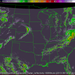
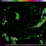
Be sure that your input index is pointing to both the forecast (HRRR) and observed (radar) fields.  The algorithm will then take all 180 min HRRR forecasts, as well as all of the radar observations, and approximate those images with Gaussians, as shown in the figures below. The algorithm will then generate error scores for corresponding HRRR and radar grids and output the scores to the file specified in the -o option of the command line.

*Note: It is important to be sure that the domains of your two grids match. This can be easily done with w2socreforecastll. Simply specify which grid you would like the other to be remapped to with the -R flag in the command line. In the images above, the HRRR field was remapped to match the domain of the radar field, and then the Gaussians were created.

An excerpt of the output file form w2scoreforecastll is below:

<iteration number="17" forecast_time="20130613-170000" target_time="20130613-200000" timedifference="180">
 <gmmComparisionScore translation_error="0.145385" rotation_error="0.00267211" scaling_error="0.51418" combined_error="0.30124" num_gmm="1"/>
 <gmmComparisionScore translation_error="0.420869" rotation_error="0.00603904" scaling_error="0.140152" combined_error="0.197544" num_gmm="2"/>
 <gmmComparisionScore translation_error="0.294767" rotation_error="0.364796" scaling_error="0.337474" combined_error="0.330126" num_gmm="6"/>
 <gmmComparisionScore translation_error="0.375277" rotation_error="0.0519002" scaling_error="0.159446" combined_error="0.202686" num_gmm="8"/>
 <gmmComparisionScore translation_error="0.173481" rotation_error="0.0684976" scaling_error="0.226473" combined_error="0.17898" num_gmm="18"/>
 <gmmComparisionScore translation_error="0.251112" rotation_error="0.394195" scaling_error="0.0955482" combined_error="0.201947" num_gmm="35"/>
 <gmmComparisionScore translation_error="0.231869" rotation_error="0.3287" scaling_error="0.072619" combined_error="0.17161" num_gmm="69"/>
 <gmmComparisionScore translation_error="0.14816" rotation_error="0.18702" scaling_error="0.0419667" combined_error="0.102835" num_gmm="137"/>
</iteration>

Going through this output, we first see that we are on iteration number 17, where each iteration is associated with a new timestep. Next we see that we are comparing the 180 minute HRRR created at 20130613-170000 and the radar composite reflectivity at 20130613-200000. Finally we have the error scores for each scale. There is a section of the output file like the one above for each timestep. At the end of the file, all of the error score are aggregated (not shown).

This type of information is particularly valuable in situations where you want to compare different forecasts. Perhaps you want to know if at a particular forecast hour, you get a better forecast from advecting radar data forward in time or from the HRRR. With w2scoreforecastll, you can score both forecasts to determine which one is better.

Tags: None

Creating Rotation Tracks using WDSS-II

How do you go about creating rotation tracks starting from Level-II radar data from NCDC?

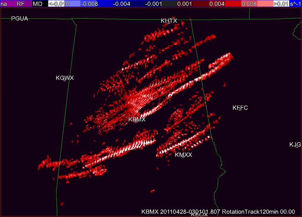
w2image-KBMX_RotationTrack120min-20110428-030101-1

The entire process is described in M. Miller, V. Lakshmanan, and T. Smith, “An automated method for depicting mesocyclone paths and intensities,” Wea. Forecasting, vol. 28, pp. 570-585, 2013

If you use Rotation Tracks in your research, please cite the above paper and also cite the papers for each of the following steps.

  1. Untar the Level-II data and place it somewhere. Let’s call this directory RAWDIR
  2. Get terrain netcdf data for your radar. You can get terrain files for US radars from ftp://ftp.nssl.noaa.gov/users/lakshman/conus_radar_blockage.tgz.   Untar this, and let’s call this directory TERRAIN
  3. Decide where you want your output products to go. Let’s call this DATADIR.
  4. Define a variable RADAR to hold your radar identifier (e.g. KBMX)
  5. Run ldm2netcdf to convert the Level-II data into NetCDF
  6. QC the radar reflectivity data.  Note that I am assuming that you have don’t have dualpol (if you do have dualpol, you should w2qcnndp) and that you do have super-resolution (if you have 1km resolution, change -R accordingly)
  7. Dealias the velocity data
  8. Compute Azimuthal Shear
  9. Run w2merger to put the data on a LatLonGrid
  10. Run w2accumulator with QC to create the rotation tracks

Here’s a script that will carry out the entire process. Edit as needed.

#!/bin/sh

RAWDIR=`pwd`/raw
RADAR=KBMX

# Overall reference about the entire process
# M. Miller, V. Lakshmanan, and T. Smith, ``An automated method for depicting mesocyclone paths and intensities,'' Wea. Forecasting, vol. 28, pp. 570-585, 2013. 

TERRAIN=~/WDSS2/gtopo30/radars/$RADAR.nc
DATADIR=`pwd`/$RADAR

# (5) convert Level-II to netcdf
# V. Lakshmanan, T. Smith, G. J. Stumpf, and K. Hondl, ``The warning decision support system - integrated information,'' Wea. Forecasting, vol. 22, no. 3, pp. 596-612, 2007.
ldm2netcdf -i $RAWDIR -o $DATADIR -s $RADAR -p $RADAR -a -1 --verbose
replaceIndex -i $DATADIR/code_index.fam -o $DATADIR/code_index.xml

# (6) note: if you have dualpol data, use w2qcnndp instead of w2qccn. The rest of the command-line is the same
# V. Lakshmanan, A. Fritz, T. Smith, K. Hondl, and G. J. Stumpf, ``An automated technique to quality control radar reflectivity data,'' J. Applied Meteorology, vol. 46, pp. 288-305, Mar 2007
# V. Lakshmanan, C. Karstens, J. Krause, and L. Tang, ``Quality control of weather radar data using polarimetric variables,'' J. Atm. Ocea. Tech., vol. 0, p. 0, 2013. 
w2qcnn -i $DATADIR/code_index.xml -o $DATADIR -R 0.25x0.5x460 -s $RADAR -E $TERRAIN -u --verbose
replaceIndex -i $DATADIR/code_index.fam -o $DATADIR/code_index.xml

# (7) note: if you have sounding information, provide it. the results will be better
# Jing and Wiener 1993
dealias2d -i $DATADIR/code_index.xml -o $DATADIR --verbose
replaceIndex -i $DATADIR/code_index.fam -o $DATADIR/code_index.xml

# (8) run LLSD
# Smith and Elmore 2004 
w2circ -i $DATADIR/code_index.xml -o $DATADIR -a -w -z ReflectivityQC -Z 20 -D -t -c -L "0:2:1.0:7.5:AGL  3:6:0:90:AGL" -V "0.5 250 920" -G $RADAR -g $TERRAIN --verbose
replaceIndex -i $DATADIR/code_index.fam -o $DATADIR/code_index.xml

# (9) run w2merger to put the data on a cartesian grid
# V. Lakshmanan, T. Smith, K. Hondl, G. J. Stumpf, and A. Witt, ``A real-time, three dimensional, rapidly updating, heterogeneous radar merger technique for reflectivity, velocity and derived products,'' Wea. Forecasting, vol. 21, no. 5, pp. 802-823, 2006. 
# V. Lakshmanan and T. W. Humphrey, ``A MapReduce technique to mosaic continental-scale weather radar data in real-time,'' IEEE J. of Select Topics in Appl. Earth Obs. and Remote Sensing, vol. 0, no. 0, 2013.
TOP=`grep -A 2 $RADAR ~/WDSS2/src/w2/w2config/misc/radarinfo.xml | head -2 | tail -1 | sed 's/[=\"]/ /g' | awk '{print $3+4,$5-4}'`
BOT=`grep -A 2 $RADAR ~/WDSS2/src/w2/w2config/misc/radarinfo.xml | head -2 | tail -1 | sed 's/[=\"]/ /g' | awk '{print $3-4,$5+4}'`
echo "$TOP to $BOT"
w2merger -i $DATADIR/code_index.xml -o $DATADIR -I AzShear_0-2kmAGL -p 0.001 -e 60 -C 1 -R 230 -t "$TOP 1" -b "$BOT 0" -s "0.005 0.005 1" --verbose
replaceIndex -i $DATADIR/code_index.fam -o $DATADIR/code_index.xml

# (10) run w2accumulator with QC
# V. Lakshmanan, M. Miller, and T. Smith, ``Quality control of accumulated fields by applying spatial and temporal constraints,'' J. Atmos. Ocean. Tech., vol. 30, pp. 745-757, 2013. 
w2accumulator -i $DATADIR/code_index.xml -o $DATADIR -R -s -t "60 120 360" -C 1 -O RotationTrack -t 120 -Q blob:0.002:0.005:25:azshear,mht:1:2:1800:5:1 -g MergedAzShear_0-2kmAGL --verbose
replaceIndex -i $DATADIR/code_index.fam -o $DATADIR/code_index.xml
Tags: None

Improved w2dualpol

As discussed in our previous post, we streamlined the WDSS-II ORPG processing into 1 algorithm, w2dualpol. In addition to this streamlining, we have also found two methods to enhance the speed at which w2dualpol can run. First, the algorithm can find a “capping tilt” and only processes the tilts below that elevation. Second, if you’re interested in only rain rates, the algorithm can determine the lowest elevation unblocked by terrain, and only process the tilts at or below that tilt.

The capping tilt is determined by reading in subsequent tilts of the radar until a tilt is found in which none of the pixels have a reflectivity greater than a user-defined threshold, set with the -m flag. The algorithm then considers this tilt the cap, and does not read any tilts above this cap. The algorithm then runs, reading in all tilts below and including the capping tilt. This continues until either a) another capping tilt is found below the current capping tilt, or b) a pixel is found in the current capping tilt with a reflectivity greater than the threshold specified by the -m flag.

If a new capping tilt is found below the current capping tilt, the algorithm will then reads only the tilts below the new capping tilt. If a pixel is found to exceed the reflectivity threshold in the current capping tilt, the algorithm resumes reading all tilts until it finds another tilt with in which the reflectivity does not exceed the threshold in any pixel, and a new capping tilt is declared.

By specifying a threshold with the -m flag, you are basically telling the algorithm that you are not interested in any echoes below this threshold. You are also assuming that if there are no pixels in which the reflectivity exceeds the threshold in a particular tilt, there are also no pixels in which the reflectivity exceeds the threshold in the tilts above.

Finally, if you are interested in only rain rates, you can set the -E flag to further reduce the time it takes this algorithm to run. Rain rates are determined by examining the pixels nearest to the ground. In a perfectly flat world, we could read in and process only the lowest tilt from the radar and greatly reduce the processing time. However, we know that our world is not perfectly flat, and that many radars have terrain blocking some of the radials at the lower tilts. For these radials blocked by terrain, we need to find the next lowest unblocked radial. Therefore, we have devised a method in which we can determine the lowest tilt unblocked by terrain for each radar. Once this tilt is determined, only data below and including that tilt needs to be processed.

You can specify that you would like to process only up to the lowest unblocked tilt by setting the -E flag to the lowest elevation angle scanned by your radar (0.5 in the case of the WSR-88D network). This needs to be specified so the algorithm knows at which elevation to start looking for the lowest unblocked tilt.

So, if you are interested in only rain rates from a radar in the WSR-88D network, your command would look like:

w2dualpol -i /data/KTLX/code_index.fam -o /data/KTLX -s KTLX -m 10 -E 0.5 -T /data/terrain/KTLX.nc --outputProducts=RREC

Notice that along with the -E flag, the -T flag is also set, specifying the terrain file for your radar. Additionally, the -m flag is set to 10, specifying that the capping elevation be set as the lowest elevation in which no pixels exceed 10 dBZ.

It should be noted that if you’re interested in processing some products at all elevations (say, HCA and MSIG), but the rain rates at only the lowest unblocked elevation, you will want to run two iterations of w2dualpol in order to process the data in the least amount of time.

First:

w2dualpol -i /data/KTLX/code_index.fam -o /data/KTLX -s KTLX -0 1 -m 10 -T /data/terrain/KTLX.nc --outputProducts=DHCA,MSIG

and then:

w2dualpol -i /data/KTLX/code_index.fam -o /data/KTLX -s KTLX -m 10 -E 0.5 -T /data/terrain/KTLX.nc --outputProducts=RREC

Through the implementation of the capping elevation and the lowest unblocked elevation, we are able to halve the processing time of w2dualpol. This means that the processing time is about 1/4 of that of the original ports of the ORPG algorithms, discussed in the previous post.

Tags: None

Streamlined ORPG dual-pol processing with w2dualpol

WDSS-II contains ports of several NWS open radar product generator (ORPG) dual-pol algorithms. Through the use of these ports, it is possible to do a multitude of things, including running the hydrometeor classification algorithm (HCA) and computing instantaneous rain fall rates from the dual-pol variables and the HCA. Previously, the only way to do this in WDSS-II required the use of multiple algorithms. This workflow for computing rain rates from dual-pol observations is:

w2dp_preproc → w2dp_hca → w2dp_rainrates

w2dp_preproc takes the base dual-pol outputs from ldm2netcdf, which tend to be noisy and difficult to interpret or use in algorithms, and recombines them from a 0.5 degree azimuthal resolution to a 1.0 degree azimuthal resolution. Through this recombination, the noise of the dual-pol products is reduced. Additionally, this algorithm creates quality flags for each product, which are required by the HCA algorithm.

Next w2dp_hca reads in all of the output from w2dp_preproc, and, you guessed it, runs the HCA. The hydrometeor classifications, as well as some of the output from w2dp_preproc, are then be passed into w2dp_rainrates to determine instantaneous rainfall rates for each dual-pol variable and the HCA. Unfortunately, this workflow is not quite fast enough to run in real-time, so we sought a way to speed it up.

This speed up is achieved by combining w2dp_preproc, w2dp_hca, and w2dp_rainrates into 1 algorithm: w2dualpol. With w2dualpol, you can process as much or as little data as you want. By default, w2dualpol will run all the way through the computational stream discussed above. However, you can specify where in the computational stream you want w2dualpol to stop with the -O flag, where;

0: Preproc — stop after the preprocessor calculations
1: HCA – stop after the HCA calculations
2: RainRates – stop after the rain rate calculations (default)

Additionally, you can specify the products you want written out with the –outputProducts flag. So, for example, if you’re only interested in the HCA, your command line would look like:

w2dualpol -i /data/KTLX/code_index.fam -o /data/KTLX -s KTLX -O 1 --outputProducts=DHCA

Or, if you’re interested in the HCA and the rain rates computed from the HCA, you can run:

w2dualpol -i /data/KTLX/code_index.fam -o /data/KTLX -s KTLX --outputProducts=DHCA,RREC
With these changes, we were able to process data in less than half the time it took to put the data through the three algorithms discussed above. We then made additional improvement to w2dualpol that sped it up even further. These improvements are discussed in our next blog post.


Tags: None

ldm2netcdf now handles SAILS correctly

The implementation of the Supplemental Adaptive Intra-Volume Low-Level Scan (SAILS) for the 88D radars presented a problem for the WDSS-II ingestor ldm2netcdf  because it relied on VCP definitions stored in XML configuration files.  Those XML files defined which elevations matched up with each tilt. However, SAILS can insert a supplemental 0.5 degree scan into the existing VCP at any time. With no changes, ldm2netcdf would incorrectly label the new 0.5 tilt as the next expected tilt as defined in its VCP XML file.

To solve this problem, ldm2netcdf now processes Message 5 in the Level-II data stream (the RDA Volume Coverage Data)  to map each incoming tilt to the correct elevation. The new 0.5 elevations get correctly labeled and saved just like any other 0.5 tilt.

Algorithms listening to 0.5 elevations will be notified of these new tilts just like normal.  Algorithms that listen to all tilts will insert them into the constantly updating virtual volume as the latest 0.5-degree tilt of data for that elevation. So, with the change to ldm2netcdf, downstream algorithms such as w2qcnndp, w2vil, w2merger, etc. deal with the SAILS tilt transparently.

If you do not want the SAILS elevation to be inserted into the data stream, you can specify the ‘-e’ option on the command line of ldm2netcdf to separate out the extra SAILS tilts. The SAILS tilts will then be saved into a separate directory, such as Reflectivity_SAILS, or AliasedVelocity_SAILS.  We do not recommend this, as you are essentially throwing away the extra information.

Finally, we took this opportunity to eliminate some outdated command line options in ldm2netcdf.  First, is the ‘-D’ option for dealiasing.  The dealiasing code in ldm2netcdf is very old and the dealias2d command provides much better results. Second, the ‘-c’ for compositing will be removed since w2vil does a much better job creating composites.

The new changes are being tested and will be rolled out when all the kinks are worked out.

VCP dependence removed from WDSS-II

In the past, in order to create a volumetric product in WDSS-II, it was required that the VCP used by the radar be known. This was not a problem for users working with data from the WSR-88D network, but for those utilizing data from outside of that network, a few extra steps were required, including the creation of a “fake” VCP file that contained the levels at which the radar had scanned.

However, the WSR-88D network recently adopted two new concepts to its scanning strategies. The Automated Volume Scan Evaluation and Termination (AVSET) concept allows any site to not perform higher-elevation scans when no storms are detected. The Supplemental Adaptive Intra-Volume Low-Level Scan (SAILS) gives radars in the 88D network the capability of adding in a supplemental 0.5 degree scan at any time.

While AVSET and SAILS have many advantages to them, the combination of these concepts have made using the VCP of a radar to help build volumetric products unreliable. Therefore, rather than depending on the VCP to build virtual volumes, we have taken the VCP dependence out of all of our products. This means that when working with data from outside of the WSR-88D network, including data from outside the US, users no longer need to create these “fake” VCP files, nor does the VCP need to be defined in the data. Users simply need to be sure that an appropriate expiry time for each scan is specified (using the ExpiryInterval attribute in the netcdf files) to ensure that old data ages off in a timely fashion.

Algorithms affected include:  w2vil and w2circ.

Cleaner, crisper rotation tracks

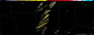
We are really happy when public safety agencies use the imagery from http://ondemand.nssl.noaa.gov/ to show the impact of the recent tornadoes in Illinois.  Hey, that’s our stuff, we want to shout. It reminds us of why we do what we do.

But there’s a lot of noise on those accumulation products, noise that can be removed by the use of Multiple Hypothesis Tracking (MHT).  We couldn’t do MHT on-demand or in real-time because it is so slow, but just a few weeks ago, we figured out a way to do it faster with not much of a tradeoff in noise removal.

We repeated the analysis of the Illinois outbreak using the faster method and boy, is it faster! We can process an hour of data in 5 minutes!  (Here are the cleaned-up rotation tracks for the Illinois tornadoes. It is a KML file, so view it in Google Earth.) MHT will be implemented on the ondemand website in a few days.  So, the next time you see folks sharing Rotation Tracks images, they will be cleaner and crisper.

Rotation Tracks today
Rotation Tracks with MHT (very, very slow)
Optimized MHT
Optimized MHT


Tags: None

w2accumulator applies MHT faster

One of the best ways to improve the quality of the Rotation Tracks products is to apply spatial QC using hysteresis and temporal QC using Multiple Hypothesis Tracking.

Unfortunately, this used to be quite slow. An hour of azimuthal shear data covering the CONUS could take as much as two hours to process. Therefore, it was used only in research studies and off-line, but not to produce the post-event rotation tracks that you can download from http://ondemand.nssl.noaa.gov/

w2accumulator’s -Q option now supports two vastly more efficient optimizations. You can specify that the number of hypothesis is 1 (meaning to only keep the best track, and not bother about second-best, third-best, etc.) or that the algorithm should retain all potential tracks (specifying -1 for number of hypotheses).  These are the most likely values that you will want to specify and with these, the algorithm runs 20x faster.  Yup, you can now process an hour of data in about 6 minutes.

Method -Q option CPU Time (microseconds)
No QC ” “ 46
5 best blob:0.002:0.005:2:azshear,mht:1:2:1800:5:5 2046
Only best blob:0.002:0.005:2:azshear,mht:1:2:1800:5:1 132
All reasonable blob:0.002:0.005:2:azshear,mht:1:2:1800:5:-1 138

You used to have only the first two options for -Q available. Now, you have two more, and these two “special” values are highly optimized.

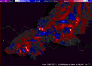
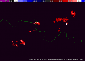
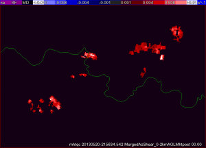
What’s the impact of these options? (Open the images in different tabs in your browser and switch between them so that you can see the differences between the last two images more readily)

w2image-input_MergedAzShear_0-2kmAGL-20130520-215833-1
Azimuthal shear field without QC
Keeping only best hypothesis
Keep all reasonable hypotheses

For more details about MHT-QC and its application to rotation tracks products, please see these scientific articles:

M. Miller, V. Lakshmanan, and T. Smith, “An automated method for depicting mesocyclone paths and intensities,” Wea. Forecasting, vol. 28, pp. 570-585, 2013.

V. Lakshmanan, M. Miller, and T. Smith, “Quality control of accumulated fields by applying spatial and temporal constraints,” J. Atmos. Ocean. Tech., vol. 30, pp. 745-757, 2013.