Improved w2dualpol

As discussed in our previous post, we streamlined the WDSS-II ORPG processing into 1 algorithm, w2dualpol. In addition to this streamlining, we have also found two methods to enhance the speed at which w2dualpol can run. First, the algorithm can find a “capping tilt” and only processes the tilts below that elevation. Second, if you’re interested in only rain rates, the algorithm can determine the lowest elevation unblocked by terrain, and only process the tilts at or below that tilt.

The capping tilt is determined by reading in subsequent tilts of the radar until a tilt is found in which none of the pixels have a reflectivity greater than a user-defined threshold, set with the -m flag. The algorithm then considers this tilt the cap, and does not read any tilts above this cap. The algorithm then runs, reading in all tilts below and including the capping tilt. This continues until either a) another capping tilt is found below the current capping tilt, or b) a pixel is found in the current capping tilt with a reflectivity greater than the threshold specified by the -m flag.

If a new capping tilt is found below the current capping tilt, the algorithm will then reads only the tilts below the new capping tilt. If a pixel is found to exceed the reflectivity threshold in the current capping tilt, the algorithm resumes reading all tilts until it finds another tilt with in which the reflectivity does not exceed the threshold in any pixel, and a new capping tilt is declared.

By specifying a threshold with the -m flag, you are basically telling the algorithm that you are not interested in any echoes below this threshold. You are also assuming that if there are no pixels in which the reflectivity exceeds the threshold in a particular tilt, there are also no pixels in which the reflectivity exceeds the threshold in the tilts above.

Finally, if you are interested in only rain rates, you can set the -E flag to further reduce the time it takes this algorithm to run. Rain rates are determined by examining the pixels nearest to the ground. In a perfectly flat world, we could read in and process only the lowest tilt from the radar and greatly reduce the processing time. However, we know that our world is not perfectly flat, and that many radars have terrain blocking some of the radials at the lower tilts. For these radials blocked by terrain, we need to find the next lowest unblocked radial. Therefore, we have devised a method in which we can determine the lowest tilt unblocked by terrain for each radar. Once this tilt is determined, only data below and including that tilt needs to be processed.

You can specify that you would like to process only up to the lowest unblocked tilt by setting the -E flag to the lowest elevation angle scanned by your radar (0.5 in the case of the WSR-88D network). This needs to be specified so the algorithm knows at which elevation to start looking for the lowest unblocked tilt.

So, if you are interested in only rain rates from a radar in the WSR-88D network, your command would look like:

w2dualpol -i /data/KTLX/code_index.fam -o /data/KTLX -s KTLX -m 10 -E 0.5 -T /data/terrain/KTLX.nc --outputProducts=RREC

Notice that along with the -E flag, the -T flag is also set, specifying the terrain file for your radar. Additionally, the -m flag is set to 10, specifying that the capping elevation be set as the lowest elevation in which no pixels exceed 10 dBZ.

It should be noted that if you’re interested in processing some products at all elevations (say, HCA and MSIG), but the rain rates at only the lowest unblocked elevation, you will want to run two iterations of w2dualpol in order to process the data in the least amount of time.

First:

w2dualpol -i /data/KTLX/code_index.fam -o /data/KTLX -s KTLX -0 1 -m 10 -T /data/terrain/KTLX.nc --outputProducts=DHCA,MSIG

and then:

w2dualpol -i /data/KTLX/code_index.fam -o /data/KTLX -s KTLX -m 10 -E 0.5 -T /data/terrain/KTLX.nc --outputProducts=RREC

Through the implementation of the capping elevation and the lowest unblocked elevation, we are able to halve the processing time of w2dualpol. This means that the processing time is about 1/4 of that of the original ports of the ORPG algorithms, discussed in the previous post.

Tags: None

Streamlined ORPG dual-pol processing with w2dualpol

WDSS-II contains ports of several NWS open radar product generator (ORPG) dual-pol algorithms. Through the use of these ports, it is possible to do a multitude of things, including running the hydrometeor classification algorithm (HCA) and computing instantaneous rain fall rates from the dual-pol variables and the HCA. Previously, the only way to do this in WDSS-II required the use of multiple algorithms. This workflow for computing rain rates from dual-pol observations is:

w2dp_preproc → w2dp_hca → w2dp_rainrates

w2dp_preproc takes the base dual-pol outputs from ldm2netcdf, which tend to be noisy and difficult to interpret or use in algorithms, and recombines them from a 0.5 degree azimuthal resolution to a 1.0 degree azimuthal resolution. Through this recombination, the noise of the dual-pol products is reduced. Additionally, this algorithm creates quality flags for each product, which are required by the HCA algorithm.

Next w2dp_hca reads in all of the output from w2dp_preproc, and, you guessed it, runs the HCA. The hydrometeor classifications, as well as some of the output from w2dp_preproc, are then be passed into w2dp_rainrates to determine instantaneous rainfall rates for each dual-pol variable and the HCA. Unfortunately, this workflow is not quite fast enough to run in real-time, so we sought a way to speed it up.

This speed up is achieved by combining w2dp_preproc, w2dp_hca, and w2dp_rainrates into 1 algorithm: w2dualpol. With w2dualpol, you can process as much or as little data as you want. By default, w2dualpol will run all the way through the computational stream discussed above. However, you can specify where in the computational stream you want w2dualpol to stop with the -O flag, where;

0: Preproc — stop after the preprocessor calculations
1: HCA – stop after the HCA calculations
2: RainRates – stop after the rain rate calculations (default)

Additionally, you can specify the products you want written out with the –outputProducts flag. So, for example, if you’re only interested in the HCA, your command line would look like:

w2dualpol -i /data/KTLX/code_index.fam -o /data/KTLX -s KTLX -O 1 --outputProducts=DHCA

Or, if you’re interested in the HCA and the rain rates computed from the HCA, you can run:

w2dualpol -i /data/KTLX/code_index.fam -o /data/KTLX -s KTLX --outputProducts=DHCA,RREC
With these changes, we were able to process data in less than half the time it took to put the data through the three algorithms discussed above. We then made additional improvement to w2dualpol that sped it up even further. These improvements are discussed in our next blog post.


Tags: None

Coordinates in WDSS-II

There seems to be some confusion about the geolocation of WDSS-II’s grids.  First of all, most of the grids produced by WDSS-II algorithms are in Plate Carree (or equirectangular) projection for the reasons ably set forth in this cartoon.

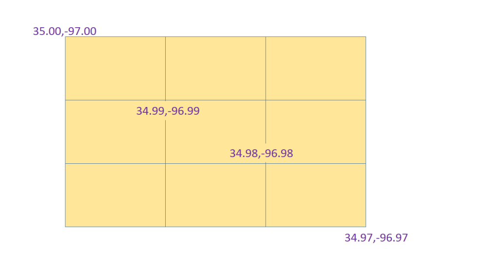
Suppose you were to ask w2merger to make you a grid from radar data and you specify the top (northwest) corner with -t and bottom (southeast) corner with -b and spacing with -s as (35,-97), (34.97, -96.97) and (0.01,0.01) respectively.  You would then get this 3×3 grid:

The grid you get if you ask w2merger for -t "35 -97" -b "34.97 -96.97"
The grid you get if you ask w2merger for -t “35 -97” -b “34.97 -96.97”

I have found that if you consider that all pixels occupy a definite area of the earth, the above representation becomes very logical. It is also intuitive in that there are 3 pixels between 35 degrees and 34.97 degrees at a spacing of 0.01 degrees.

In the netcdf files output by WDSS-II, you will find that the northwest corner and the grid spacing for the above grid would be encoded as (35,-97) and (0.01,0.01).

So, are the pixels in WDSS-II defined by their north-west corners? Unfortunately, no. For that, you have to take into account that while a pixel occupies a certain area, it has only one value. Which location within the pixel does that value correspond to? The value of a bin is the average value within the region covered by that bin.

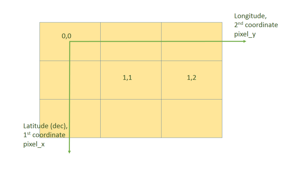
The answer to the second question leads to some tricky semantics. Before we get to those, let’s move on from the world geographic system to the projected coordinate system of the grid itself (see ArcGIS for an explanation of the difference).  Because the projection in question is Platee Carree, the transformation is a simple linear one between pixel coordinates and latitude-longitude, but such a transformation exists. For this coordinate system, the (0,0) point is the center of the northwest grid point.  This is needed so that we can think of a pixel’s value as being the average value within the bin if we had somehow had infinite resolution. The grid’s coordinate system, to put a picture to it, is like this:

Projected coordinate system

A couple of things may warrant noting. The first coordinate (the slower-changing one) is the latitude direction and the second coordinate (the faster changing one) is the longitude one. In other words, grid values are written starting from the northwest corner in rows.  Confusingly, the first coordinate (the “vertical” one if you are staring at an image) is called the x-axis in the sparse-grid netcdf format (“pixel_x”) and is the coordinate we ask for first on all command-lines that ask for a position or length.  [Side note: This is because my background is in image processing and linear algebra where this right-handed coordinate system is common. By the time I figured out that meteorologists and computer graphics used “x” for the “horizontal” dimension, it was too late and there was too much code written with the matrix notation firmly in place.]

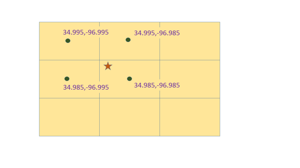
The two definitions above are very intuitive, and if you don’t think much about it, you will probably end up doing the right thing. But just to make sure you are thinking about this the right way, try to answer this question.  Given the grid above, what is the value at the location denoted by a star in this diagram?

To get the value at the location denoted by the star, you would interpolate the 4 pixels closest to the star and assign weights to those values that depend on the distance between the star and the centers of those pixels
To get the value at the location denoted by the star, you would interpolate between the values at the 4 pixels closest to the star. The weights of each of these values would depend on the distance between the star and the centers of the corresponding pixels

To find the nearest neighbor to a point (lat,lon) you would start by computing floor( (nwlat-lat)/deltalat ) to get the first pixel coordinate and floor( (lon-nwlon)/deltalon ) to get the second pixel coordinate.  If you wished to interpolate, you would also compute the ceil() besides computing the floor() so that you get the four pixels in question. Then, you would compute the distance of the stars from the pixel centers to get distance-weights and then compute a weighted average of the four values.


Tags: None