Using GMMs to score gridded forecasts with w2scoreforecastll

Determining how closely a forecast matches what happens in reality is a crucial step in the evaluation of any type of forecast. Gridded forecasts, which are of particular interest to WDSS-II users, are no different. With this in mind, we will cover a method in WDSS-II to compare gridded forecasts to gridded observations. To make this comparison, we will make use of the algorithm w2scoreforecastll, which creates scores for the gridded forecasts based on how well they match observations.

More generally, w2scoreforecastll is used to compare two supposedly equivalent 2D fields (e.g., a forecast field and an observation field). The algorithm quantifies just how different the two fields are through an error score. When the error score is low, the two grids match well, meaning that the forecast did a good job of approximating reality.

In w2scoreforecastll, there are 4 different methods by which you can generate scores for your forecasts:

  1. Pixel By Pixel: Just comparing the values in corresponding pixels in each grid
  2. Object By Object: Used to score forecasted objects (e.g., storms)
  3. Gaussian Mixture Models: Described below
  4. Probabilistic: Used to score probabilistic forecasts

In many instances, the best option for scoring gridded forecasts is option number 3, Gaussian Mixture Models. This method is outlined in great detail in  V. Lakshmanan and J. Kain, A Gaussian mixture model approach to forecast verification, Wea. Forecasting, vol. 25, no. 3, pp. 908-920, 2010.

In a nutshell, this algorithm approximates both the forecasted and observed grids with a mixture of Gaussians. Based on the parameters of these Gaussians, the algorithm computes 3 different measures of error: 1) translation error, 2) rotation error, and 3) scaling error. These errors are then all incorporated into one measure of error for the forecast, the combined error.

These error scores are computed at 8 different spatial scales. At the coarsest scale, the grids are approximated by just 1 Gaussian. Then, at subsequently finer scales, the number of Gaussians used to approximate the grids increases roughly exponentially to about 128 Gaussians at the finest scale.

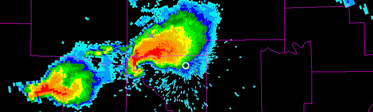
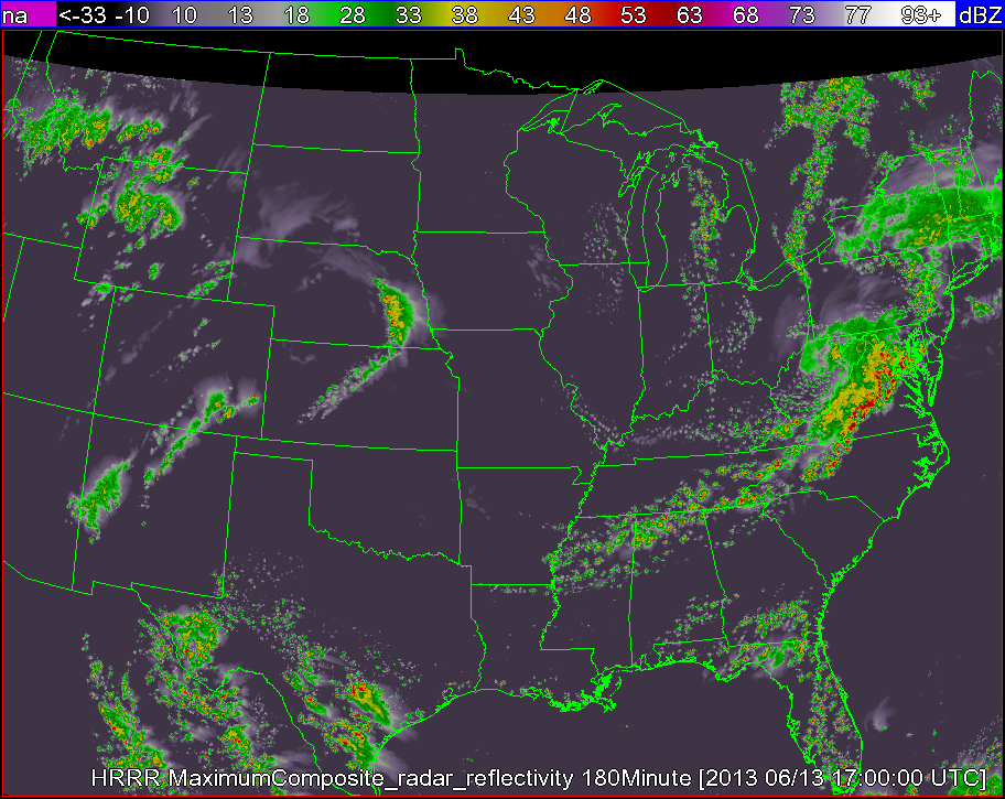
As an example, lets say we are interested in seeing how close the 180 minute composite reflectivity from the High Resolution Rapid Refresh (HRRR) numerical forecast model gets to reality (here, we will say that the merged composite reflectivity from the WSR-88D network is reality). To do this, just use the command:

w2scoreforecastll -i /localdata/20130613/score_index.xml -o /localdata/20130613/HRRR/180minute/score.out -T "MergedReflectivityQCComposite:00.00 -F MaximumComposite_radar_reflectivity:180Minute -t 180 -m 3 -R Tracked

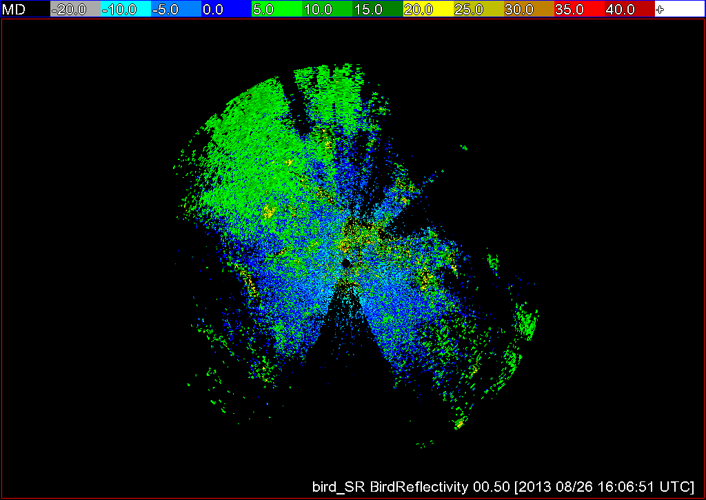
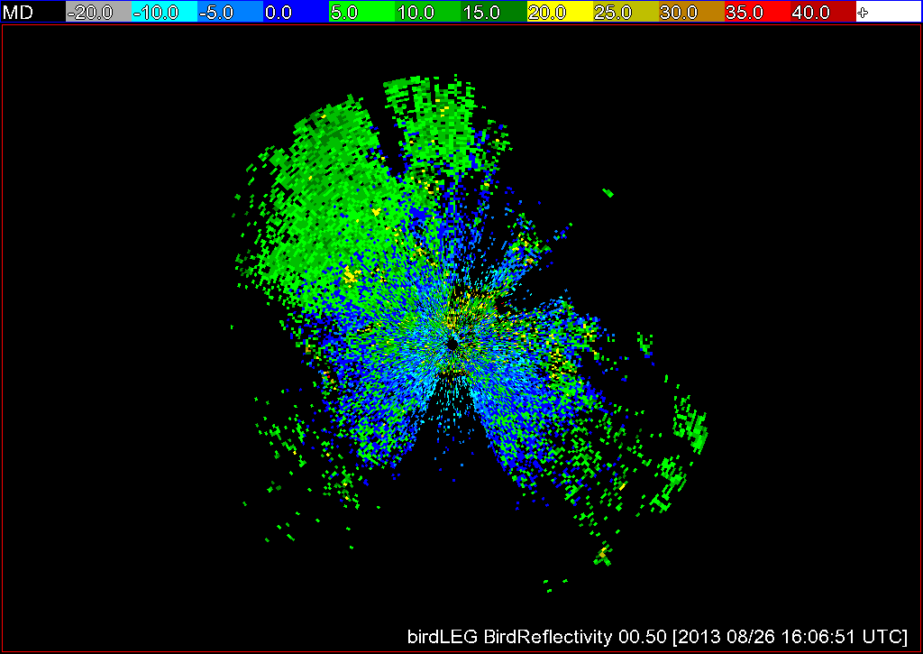
Be sure that your input index is pointing to both the forecast (HRRR) and observed (radar) fields.  The algorithm will then take all 180 min HRRR forecasts, as well as all of the radar observations, and approximate those images with Gaussians, as shown in the figures below. The algorithm will then generate error scores for corresponding HRRR and radar grids and output the scores to the file specified in the -o option of the command line.

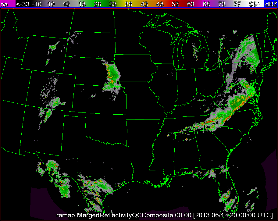
*Note: It is important to be sure that the domains of your two grids match. This can be easily done with w2socreforecastll. Simply specify which grid you would like the other to be remapped to with the -R flag in the command line. In the images above, the HRRR field was remapped to match the domain of the radar field, and then the Gaussians were created.

An excerpt of the output file form w2scoreforecastll is below:

<iteration number="17" forecast_time="20130613-170000" target_time="20130613-200000" timedifference="180">
 <gmmComparisionScore translation_error="0.145385" rotation_error="0.00267211" scaling_error="0.51418" combined_error="0.30124" num_gmm="1"/>
 <gmmComparisionScore translation_error="0.420869" rotation_error="0.00603904" scaling_error="0.140152" combined_error="0.197544" num_gmm="2"/>
 <gmmComparisionScore translation_error="0.294767" rotation_error="0.364796" scaling_error="0.337474" combined_error="0.330126" num_gmm="6"/>
 <gmmComparisionScore translation_error="0.375277" rotation_error="0.0519002" scaling_error="0.159446" combined_error="0.202686" num_gmm="8"/>
 <gmmComparisionScore translation_error="0.173481" rotation_error="0.0684976" scaling_error="0.226473" combined_error="0.17898" num_gmm="18"/>
 <gmmComparisionScore translation_error="0.251112" rotation_error="0.394195" scaling_error="0.0955482" combined_error="0.201947" num_gmm="35"/>
 <gmmComparisionScore translation_error="0.231869" rotation_error="0.3287" scaling_error="0.072619" combined_error="0.17161" num_gmm="69"/>
 <gmmComparisionScore translation_error="0.14816" rotation_error="0.18702" scaling_error="0.0419667" combined_error="0.102835" num_gmm="137"/>
</iteration>

Going through this output, we first see that we are on iteration number 17, where each iteration is associated with a new timestep. Next we see that we are comparing the 180 minute HRRR created at 20130613-170000 and the radar composite reflectivity at 20130613-200000. Finally we have the error scores for each scale. There is a section of the output file like the one above for each timestep. At the end of the file, all of the error score are aggregated (not shown).

This type of information is particularly valuable in situations where you want to compare different forecasts. Perhaps you want to know if at a particular forecast hour, you get a better forecast from advecting radar data forward in time or from the HRRR. With w2scoreforecastll, you can score both forecasts to determine which one is better.

Tags: None

Environmental information in w2dualpol

In order to run the hydrometer classification algorithm (HCA) and melting layer detection algorithm (MLDA) in w2dualpol, a “first guess” at the melting layer is required. Previously, the same default first guess was used for all radars. Obviously this solution is not ideal, as on any given day, the melting layer is likely to vary wildly across different radar sites (not to mention that at any given radar site, the melting layer is likely to vary wildly across different days).

For a better solution, you can now pull environmental information (specifically, the 0C wet bulb temperature height) into w2dualpol for a more realistic first guess at the melting layer. This first guess is provided through the use of a SoundingTable. The SoundingTable can be created in one of three ways: (1) The WDSS-II program nse can create this from a RUC analysis field.  (2) The ingest_sounding.pl script reads and converts sounding data from the U. Wyoming website into WDSS-II’s XML format. (3) You can write your own XML table file.

Once you have your SoundingTable, you will want to be sure that it is included in your RadarIndex. Then, in the command for w2dualpol, set the -S flag, and from there the algorithm will use the SoundingTable information to create a first guess at a melting layer. Additionally, the melting layer found from the SoundingTable will be used in instances when the data is not sufficient for the MLDA to run.

It should be noted that once the SoundingTable is greater than 1 day older than the radar data being processed, the SoundingTable will be aged off and the default melting layer will be used. On a related note, we have altered the algorithm such that if more than two hours pass after the MLDA has run, the algorithm will revert to using the melting layer found in the SoundingTable.

A few final notes; If a SoundingTable is present in the RadarIndex but you do not wish to use it, set -S junk and the default value will be used for the melting layer. Additionally, if no SoundingTable is available, there is no need to set -S.

Tags: None

User defined resolution in w2birddensity

A secondary use of weather radars is to detect biological scatterers such as birds, bats, and insects. When birds are detected, the echoes returned to the radar can be used to estimate the density of birds on the ground. This information is valuable in a number of situations, such as when attempting to determine where birds stop while in their migratory journey.

The algorithm w2birddensity, which is based on an algorithm described in detail here, estimates the bird density from radar reflectivity data. This is done by computing a vertical profile of reflectivity (VPR) and making adjustments to the raw reflectivity field based off of the VPR.

Previously, w2birddensity was carried out at a fixed resolution, but we have now given users the option of defining the resolution of their radar data with the -R flag. As with many of our other algorithms, just specify the gate size in km, the radial size in degrees, and the range in km, as shown below. Additionally, we have given the user the option of specifying that they would like more then the default of 5 tilts processed. This is done by setting the -n flag to the number of tilts desired.

w2birddensity -i /localdata/birddensity/code_index.xml -o /tmp/birds -s KAKQ -E ~/WDSS2/gtopo30/radars -R 0.25x0.5x100 -n 5 --verbose
birdSR
Bird reflectivity from KIWA at super-resolution.
BirdLEG
Bird reflectivity from KIWA at legacy resolution.


Tags: None

Improved w2dualpol

As discussed in our previous post, we streamlined the WDSS-II ORPG processing into 1 algorithm, w2dualpol. In addition to this streamlining, we have also found two methods to enhance the speed at which w2dualpol can run. First, the algorithm can find a “capping tilt” and only processes the tilts below that elevation. Second, if you’re interested in only rain rates, the algorithm can determine the lowest elevation unblocked by terrain, and only process the tilts at or below that tilt.

The capping tilt is determined by reading in subsequent tilts of the radar until a tilt is found in which none of the pixels have a reflectivity greater than a user-defined threshold, set with the -m flag. The algorithm then considers this tilt the cap, and does not read any tilts above this cap. The algorithm then runs, reading in all tilts below and including the capping tilt. This continues until either a) another capping tilt is found below the current capping tilt, or b) a pixel is found in the current capping tilt with a reflectivity greater than the threshold specified by the -m flag.

If a new capping tilt is found below the current capping tilt, the algorithm will then reads only the tilts below the new capping tilt. If a pixel is found to exceed the reflectivity threshold in the current capping tilt, the algorithm resumes reading all tilts until it finds another tilt with in which the reflectivity does not exceed the threshold in any pixel, and a new capping tilt is declared.

By specifying a threshold with the -m flag, you are basically telling the algorithm that you are not interested in any echoes below this threshold. You are also assuming that if there are no pixels in which the reflectivity exceeds the threshold in a particular tilt, there are also no pixels in which the reflectivity exceeds the threshold in the tilts above.

Finally, if you are interested in only rain rates, you can set the -E flag to further reduce the time it takes this algorithm to run. Rain rates are determined by examining the pixels nearest to the ground. In a perfectly flat world, we could read in and process only the lowest tilt from the radar and greatly reduce the processing time. However, we know that our world is not perfectly flat, and that many radars have terrain blocking some of the radials at the lower tilts. For these radials blocked by terrain, we need to find the next lowest unblocked radial. Therefore, we have devised a method in which we can determine the lowest tilt unblocked by terrain for each radar. Once this tilt is determined, only data below and including that tilt needs to be processed.

You can specify that you would like to process only up to the lowest unblocked tilt by setting the -E flag to the lowest elevation angle scanned by your radar (0.5 in the case of the WSR-88D network). This needs to be specified so the algorithm knows at which elevation to start looking for the lowest unblocked tilt.

So, if you are interested in only rain rates from a radar in the WSR-88D network, your command would look like:

w2dualpol -i /data/KTLX/code_index.fam -o /data/KTLX -s KTLX -m 10 -E 0.5 -T /data/terrain/KTLX.nc --outputProducts=RREC

Notice that along with the -E flag, the -T flag is also set, specifying the terrain file for your radar. Additionally, the -m flag is set to 10, specifying that the capping elevation be set as the lowest elevation in which no pixels exceed 10 dBZ.

It should be noted that if you’re interested in processing some products at all elevations (say, HCA and MSIG), but the rain rates at only the lowest unblocked elevation, you will want to run two iterations of w2dualpol in order to process the data in the least amount of time.

First:

w2dualpol -i /data/KTLX/code_index.fam -o /data/KTLX -s KTLX -0 1 -m 10 -T /data/terrain/KTLX.nc --outputProducts=DHCA,MSIG

and then:

w2dualpol -i /data/KTLX/code_index.fam -o /data/KTLX -s KTLX -m 10 -E 0.5 -T /data/terrain/KTLX.nc --outputProducts=RREC

Through the implementation of the capping elevation and the lowest unblocked elevation, we are able to halve the processing time of w2dualpol. This means that the processing time is about 1/4 of that of the original ports of the ORPG algorithms, discussed in the previous post.

Tags: None

Streamlined ORPG dual-pol processing with w2dualpol

WDSS-II contains ports of several NWS open radar product generator (ORPG) dual-pol algorithms. Through the use of these ports, it is possible to do a multitude of things, including running the hydrometeor classification algorithm (HCA) and computing instantaneous rain fall rates from the dual-pol variables and the HCA. Previously, the only way to do this in WDSS-II required the use of multiple algorithms. This workflow for computing rain rates from dual-pol observations is:

w2dp_preproc → w2dp_hca → w2dp_rainrates

w2dp_preproc takes the base dual-pol outputs from ldm2netcdf, which tend to be noisy and difficult to interpret or use in algorithms, and recombines them from a 0.5 degree azimuthal resolution to a 1.0 degree azimuthal resolution. Through this recombination, the noise of the dual-pol products is reduced. Additionally, this algorithm creates quality flags for each product, which are required by the HCA algorithm.

Next w2dp_hca reads in all of the output from w2dp_preproc, and, you guessed it, runs the HCA. The hydrometeor classifications, as well as some of the output from w2dp_preproc, are then be passed into w2dp_rainrates to determine instantaneous rainfall rates for each dual-pol variable and the HCA. Unfortunately, this workflow is not quite fast enough to run in real-time, so we sought a way to speed it up.

This speed up is achieved by combining w2dp_preproc, w2dp_hca, and w2dp_rainrates into 1 algorithm: w2dualpol. With w2dualpol, you can process as much or as little data as you want. By default, w2dualpol will run all the way through the computational stream discussed above. However, you can specify where in the computational stream you want w2dualpol to stop with the -O flag, where;

0: Preproc — stop after the preprocessor calculations
1: HCA – stop after the HCA calculations
2: RainRates – stop after the rain rate calculations (default)

Additionally, you can specify the products you want written out with the –outputProducts flag. So, for example, if you’re only interested in the HCA, your command line would look like:

w2dualpol -i /data/KTLX/code_index.fam -o /data/KTLX -s KTLX -O 1 --outputProducts=DHCA

Or, if you’re interested in the HCA and the rain rates computed from the HCA, you can run:

w2dualpol -i /data/KTLX/code_index.fam -o /data/KTLX -s KTLX --outputProducts=DHCA,RREC
With these changes, we were able to process data in less than half the time it took to put the data through the three algorithms discussed above. We then made additional improvement to w2dualpol that sped it up even further. These improvements are discussed in our next blog post.


Tags: None

Reading in HRRR files

There are many occasions in which it is useful to read model data into WDSS-II. Often times, this data comes from the RUC/RAP model, and gribToNetcdf makes it very simple to get this data in a format readable by most of the other WDSS-II algorithms. However, if you are interested in using data from the higher resolution HRRR model, reading in the data is not quite so straightforward.

In order get HRRR data into a format readable by WDSS-II, you must first create a configuration file specifying which meteorological variables you are interested in.The reason the configuration file is created is simply to save time and space. Each HRRR file contains over 100 variables. If you’re interested in only a few of the variables, why waste valuable processing time and space reading in data you are not interested in?

While this all may seem rather cumbersome at first, it’s actually not too difficult. Just follow the steps below, and you will be working with HRRR data in no time.

  1. First of all, you need to make sure you have 2 environment variables set correctly. JAVA_HOME needs to be set to the location of your java instillation, and WDSSII_INSTALL_DIR needs to be set to the wdssiijava directory.
  2. Copy the file wdssiijava/example/griddataingest.xml into the current directory, and rename it hrrr.xml.
  3. Edit hrrr.xml. The inputDir and outputDir variables must be changed to match where your data is. The filenamePatterns variable must also be changed to match something in your input files (i.e., if all of your files are named 20130106_****, you could set filenamePatterns equal to “2013”). Finally, the listVariables variable needs to be uncommented and set to “true”.
  4. Run: ./w2java.sh org.wdssii.ncingest.GridDatasetIngest ./hrrr.xml. This will create your configuration file, varList.xml. This file will contain all of the meteorological variables in your HRRR data.
  5. Edit varList.xml. For all variables that you are interested in utilizing, you will need to set them from “false” to “true” inside of varList.xml.
  6. Edit hrrr.xml. Set listVariables to false.
  7. Run ./w2java.sh org.wdssii.ncingest.GridDatasetIngest ./hrrr.xml once more, and voila, your netcdf HRRR files will be waiting for you in the directory that you specified.

For future processing, you will simply need to change the inputDir and outputDir variables in hrrr.xml. If you are interested in processing different or additional variables, simply change those variables from “false” to “true” in varList.xml.

In order to use wdssiijava, you need to have Java 7 or higher installed and in your PATH.

VCP dependence removed from WDSS-II

In the past, in order to create a volumetric product in WDSS-II, it was required that the VCP used by the radar be known. This was not a problem for users working with data from the WSR-88D network, but for those utilizing data from outside of that network, a few extra steps were required, including the creation of a “fake” VCP file that contained the levels at which the radar had scanned.

However, the WSR-88D network recently adopted two new concepts to its scanning strategies. The Automated Volume Scan Evaluation and Termination (AVSET) concept allows any site to not perform higher-elevation scans when no storms are detected. The Supplemental Adaptive Intra-Volume Low-Level Scan (SAILS) gives radars in the 88D network the capability of adding in a supplemental 0.5 degree scan at any time.

While AVSET and SAILS have many advantages to them, the combination of these concepts have made using the VCP of a radar to help build volumetric products unreliable. Therefore, rather than depending on the VCP to build virtual volumes, we have taken the VCP dependence out of all of our products. This means that when working with data from outside of the WSR-88D network, including data from outside the US, users no longer need to create these “fake” VCP files, nor does the VCP need to be defined in the data. Users simply need to be sure that an appropriate expiry time for each scan is specified (using the ExpiryInterval attribute in the netcdf files) to ensure that old data ages off in a timely fashion.

Algorithms affected include:  w2vil and w2circ.