One of the things that we’re looking at this year in the SFE is forecasting the coverage and the intensity of individual severe hazards – tornadoes, hail, and wind. Ongoing work at SPC has shown that there is some intensity information within the coverage probabilities, and the aim of this aspect of the experiment is to determine how best to unlock that information.

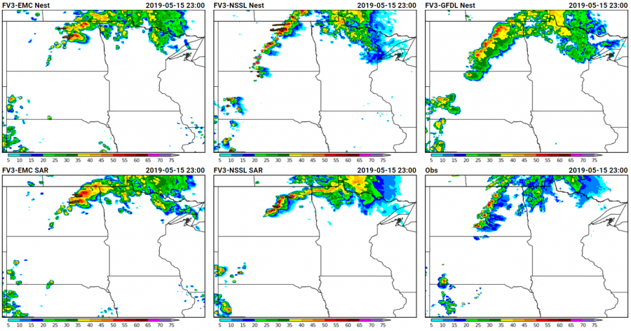
Yesterday, 16 May, provided an interesting case for the conditional intensity forecasts. CAM guidance yesterday was indicating the possibility of rotating, discrete storms across parts of North Dakota, but the location of where CAPE, shear, and the cold front would intersect left questions about the mode of convection and whether or not significant hail would be possible with these given storms. CAM guidance showed the location and progression of the storms quite well, including several experimental FV3-based CAMs that we’re looking at in the experiment.

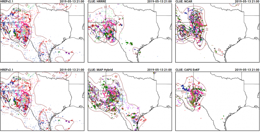
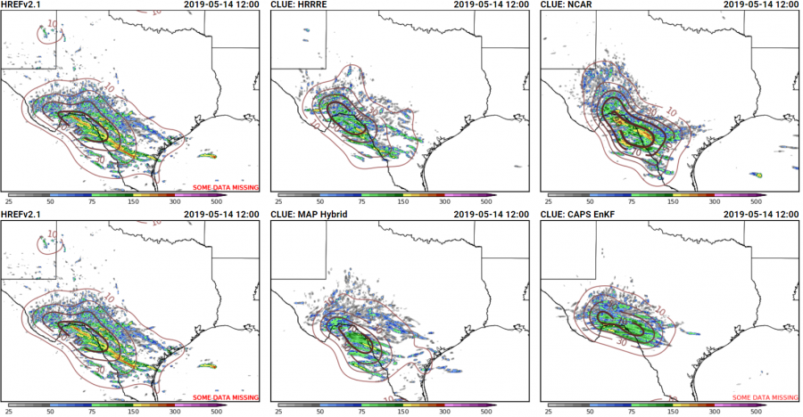
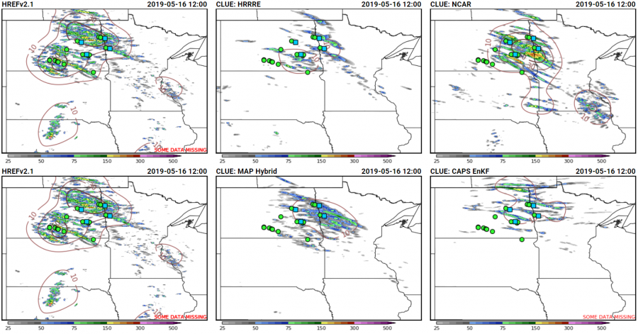
The intensity potential may have been covered better by the ensembles, and showed that a range of outcomes were possible. The 24-h maximum UH fields from several experimental ensembles showed very different depictions of the potential storm severity:

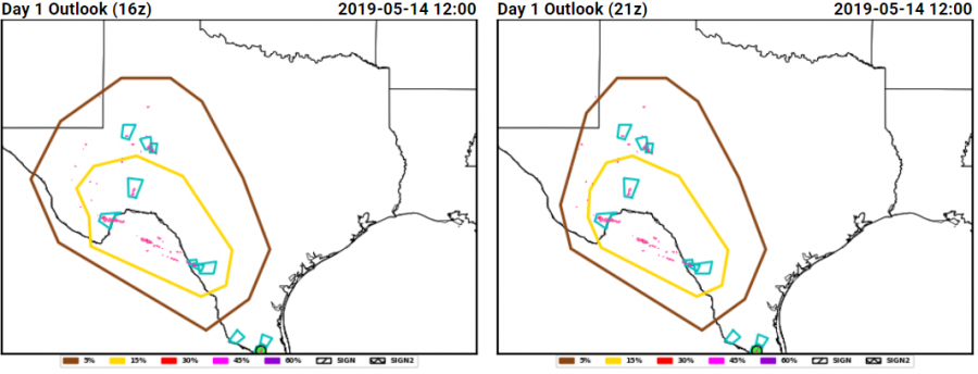
The hail forecasts from the severe hazards desk combined this guidance with environmental analysis information focusing on where the juxtaposition of shear and CAPE would be greatest, and produced probabilistic forecasts that highlighted the area where the largest density of hail forecasts occurred:

This series of forecasts was made (from left to right) the day before the event, the morning of the event, and the afternoon of the event, and shows how the severe hazards desk was able to hone in on the area at risk and reduce the false alarm area, both between Day 2 and the Day 1 outlook issued in the morning, and between the morning and afternoon Day 1 outlooks. Initially, the 15% contour was tailored the most between the Day 2 and Day 1, reducing false alarm across Minnesota. Then, between the initial forecast and the update, the western extent of the probabilities was trimmed as it became evident where the boundary forcing the convection would be.

Additionally, the forecast here not to indicate a threat of significant hail was far from straightforward. Thinking was that storms would remain discrete, especially on the southern end of the line, and could possess rotation. However, we were not confident that the environment could support the production of severe hail, and so decided to forego introducing areas of significant hail. Given the lack of significant hail reports and greater than or equal to 2″ hail in the MESH, this decision was a good one.

This week’s cases have thus far provided interesting challenges, showing differences between CAM behavior in weakly forced situations and with less-than-ideal environmental parameters. Cases like these are critical in understanding how we can best utilize the CAMs to increase forecaster capability in situations where the solutions are far from evident.

Well, the theme of the first two weeks of the experiment has been convection, convection, convection! True, this is the theme of all of the Spring Forecasting Experiments, but it has been rare in recent years to have such continuously busy weather throughout the first two weeks of the experiment. Most days thus far, convection is ongoing when we first enter the HWT at 8:00 AM. Multiple times during the first week and a half there have been watches or warnings from the NWS within the area that we’re forecasting for as we walk in the door.

Obviously, this produces a few challenges! First, we have to worry about the severity of the ongoing convection and whether it will strengthen, weaken, or continue on at its current intensity. Second, we have to concern ourselves with the potential for recovery behind an initial round of convection. Finally, we need to worry about storms will develop elsewhere in the domain, ensuring that the ongoing convection doesn’t take all of our attention. While we limit our area of responsibility to a regional domain within the CONUS, we have still faced this problem multiple times within the SFE thus far and occasionally have had issues keeping track of all of the areas of storms within our regions. Even the lower-end severe days, like yesterday, have existing precipitation that we need to determine the evolution of.

Luckily, we have expert forecasters and experimental guidance to help us determine how the convection will evolve. Several ensembles of the experimental convection-allowing models (CAMs) gave useful guidance yesterday, helping us determine the convective mode, timing, and intensity of convection.

One type of plot we examine is the paintball plot, which shows areas of high reflectivity from each ensemble member. It gives us clues to the convective mode, which can help determine what sort of severe hazard we can expect. Here’s an example of the paintballs from yesterday from five different ensemble subsets, with the observed reflectivity overlaid in the hot pink contours:

Though they may look like Jackson Pollock paintings, if you focus on one color you can start to pick out areas of discrete storms as well as areas that look like small line segments. Going through the hours, the linear structures in most ensembles progressed to the east or southeast, while cellular modes remained to the south. While these plots demonstrate what the radar may look like, it doesn’t always give insight to the severity of the storms. The updraft helicity (or UH) has been determined to be a good proxy for severe weather, so we also consider the 4-h maximum UH and the probability of UH exceeding a threshold. Yesterday, we didn’t see much in the reflectivity paintball plots that would indicate severe weather, but the UH told somewhat of a different story!

Those continuous swaths of high UH coming out of Mexico into Texas definitely caught our attention, and our forecasts reflect that there was a chance of a supercell moving across the border into Texas after initiating off of the high terrain. The UH prompted us to take a second look at the mode in the reflectivity plots, confirming that discrete supercells were a possibility.

Sure enough, a discrete supercell moved into Texas, and produced large radar-indicated Maximum Estimated Size of Hail (MESH). When we are in areas with low population, we use MESH to provide a secondary verification source in addition to Local Storm Reports (LSRs), and also look at warnings issued by the local NWS Weather Forecast Offices. Warnings indicate that an expert forecaster saw enough of a threat to warn the public of impending severe weather.

While the only hail LSR occurred across the southern part of Texas, the presence of several warnings and MESH tracks indicating hail greater than 1″ led to these forecasts being rated pretty well by the participants.

With so much convection to examine, even on the more marginal days, we have had a lot of activity in the SFE so far this year. And more looks to be on the horizon! The CAMs will likely provide plenty of convective scenarios in the coming weeks to test their capabilities.