Today we focused on the slight risk across the southeast, specifically WFO Jackson, MS. During the afternoon hours, a small linear complex was coming across northern LA towards Jackson’s CWA. Right before the CWA line, there was a wind report of snapped tree limbs of 3” diameter from Monroe Airport. There was also a measured gust from the airport of 41 mph. The velocity on radar had ~60 knot outbound winds at around 14,000 – 15,000 feet, which easily could have produced a few severe gusts to the surface. The gifs below show the linear line of storms and the associated velocity as the system moved over Monroe Airport in northeast LA with the wind report at 1952z and then continued to enter western MS.

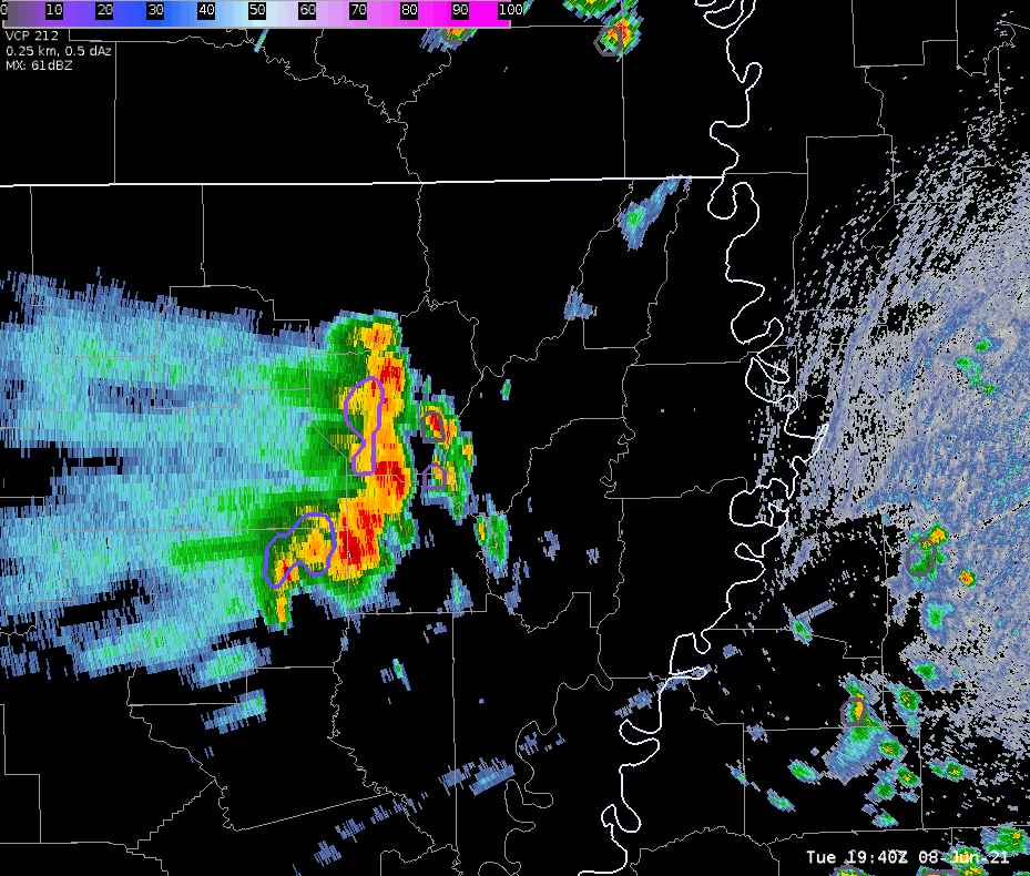
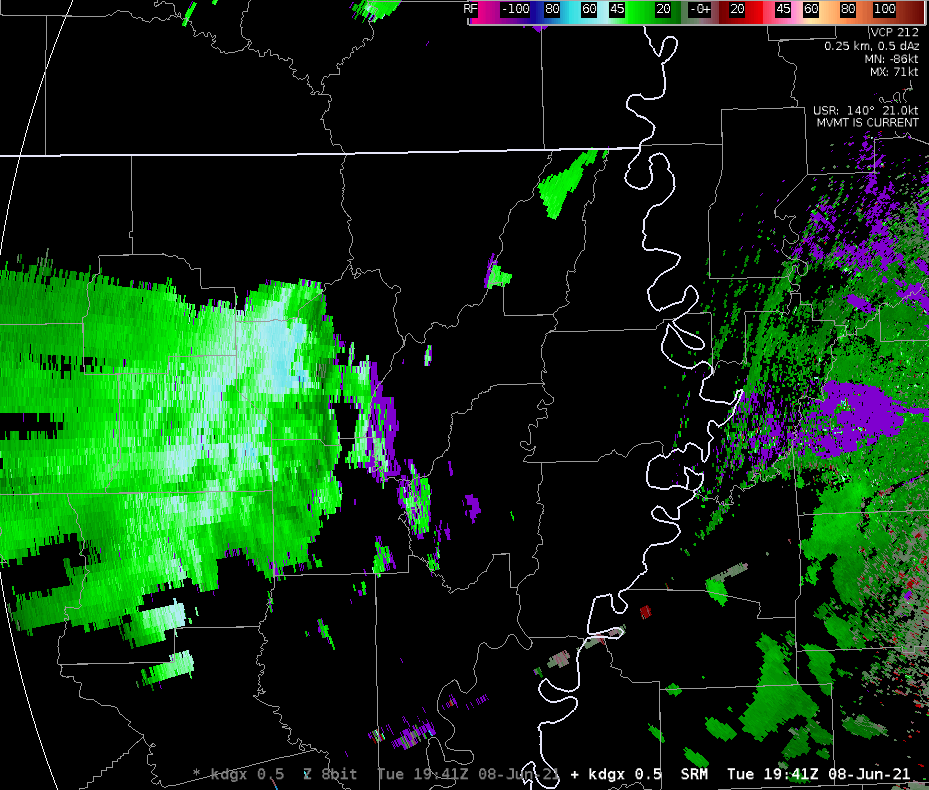
Image 1 shows a loop of radar reflectivity with prob severe overlaid and Image 2 shows the velocity associated with the radar loop.

In this situation, prob severe was not doing as good of a job on picking up on these “stronger” winds. Image 3 below shows the time of the wind damage report and 41 mph gust at the airport in northeast LA, but prob severe and prob wind are both only picking up about 20% probability of this potential. Almost two hours later, the line of storms are a bit weaker on reflectivity but just as strong or even stronger on velocity. Note, the storms were also closer to the radar at Image 4, so the stronger outbound velocities were closer to the surface. So this led to wondering is prob severe a good indicator for straight line winds?

Prob severe utilizes azimuthal shear which as seen in the Images 3 and 4 below are not present with solely outbound velocities and little to no inbound present. This is common for straight line wind scenarios, but not super helpful in terms of how prob wind is calculated. Also, the prob severe is an object oriented product that utilizes reflectivity for these objects. In this scenario, the reflectivity definitely began to weaken but velocity did not. The toughest part was the prob severe began to decrease over the two hour time span shown above, but yet several damaging wind reports of roofs blown off and trees/power lines down led me to believe the probability of prob wind should have remained constant or increased over time.

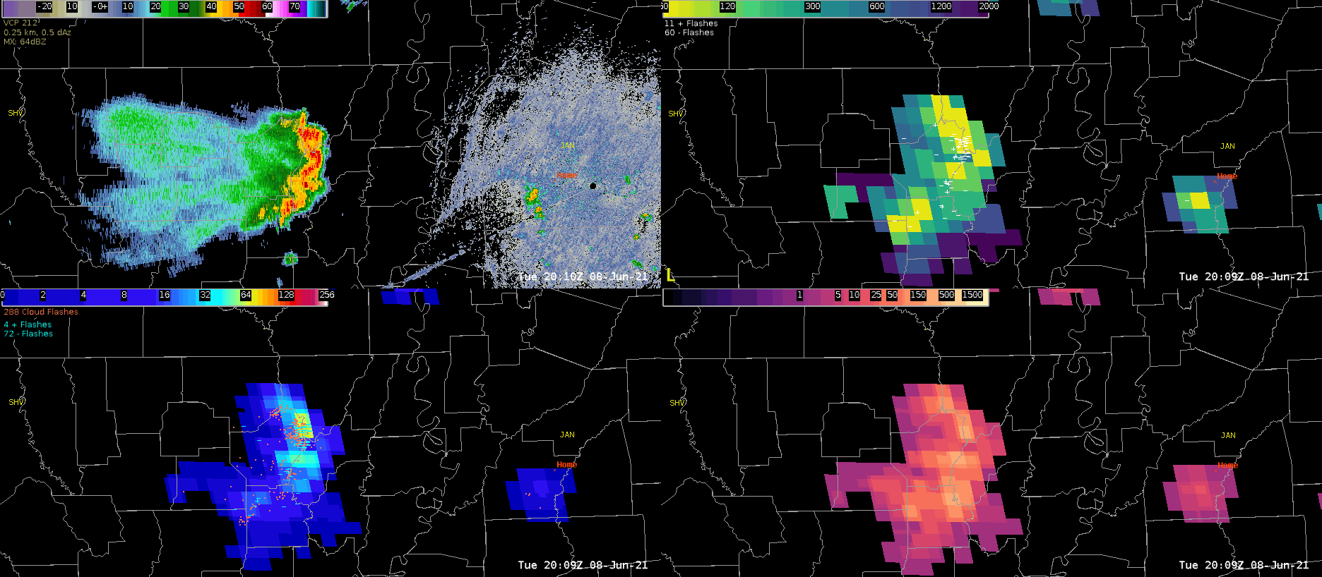
While investigating the prob severe I also took a look into the lightning characteristics within the line as you can see in the GIF below (Image 5) that there is the formation of some trailing stratiform on reflectivity. A still image was taken (Image 6) to show how the lightning began to extend westward into the light stratiform. The flash area (top right of the four panel) shows the darker purple color extending westward, which indicates the storm mode is more of that light stratiform rain with longer flashes extending through it rather than the intense small flashes within the leading line. This can be helpful in time when you may have a DSS event and the main line has passed through, but lightning is still present in the trailing light rain. Pairing the ground networks with the GLM extent and area allows a forecaster to give DSS on the latest CG stroke within the large area.

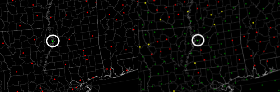
Lastly, there was a NUCAPS CONUS NOAA-20 satellite pass at around 19z, which was well before the line of storms made it to the western Jackson CWA line. No special radiosonde launches were made by local offices, so the next best observational guess of the atmospheric profile would be from satellite. Model soundings were also available to compare at the time. A RAP sounding at 19z was taken just east of the western MS border (see Image 7 below for location of this sounding) and a very nearby NUCAPS sounding was also retrieved for comparison (see Image 8 below for location of this sounding).

The soundings (Image 9 and 10 below) looked fairly similar between the model and satellite profiles; however, there were several major differences that played a key role in changing the instability parameters. The NUCAPS sounding was still slightly too low of a surface temperature with 86 deg F versus the RAP’s 89 deg F. Surface observations from 19z at that location showed a temperature of  around 91 deg F. Also, the surface dewpoint was far too low on the NUCAPS profile at the surface as it was 5 degrees below the current observation at 19z. Meanwhile, the RAP was only one degree lower than the current surface dewpoint. These subtle differences caused significant variations in the CAPE values.

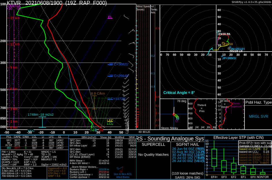
After realizing the NUCAPS profile was not accurately depicting the surface temperature/dewpoint, I decided to see what the modified sounding might look like through NSHARP. Image 11 below shows the modified NUCAPS sounding through NSHARP with a much cooler surface temperature of near 80 deg F. This was almost 10 deg below the actual surface temperatures and 6 deg below the original NUCAPS profile. The boundary layer was not representative due to this drastic difference and therefore the modified sounding had to be thrown out of the comparison.

Lastly, with knowing the line of storms were headed into the area of interest I decided to see how the forecast products were looking. Unfortunately, I did not get to save the images off in time as the forecast images disappear from AWIPS when the next pass occurs. So I was left with the web-browser version which is only in a gridded format. Unfortunately it is very difficult to depict changes in this format, whereas in AWIPS you can interpolate the image and smooth the results for a more concise display of values. Image 13 shows the comparison of the web-browser gridded format versus the AWIPS smoothed version for the West Coast pass of the NOAA-20 satellite.

– Harry Potter